Let us see how it works. In this first simulation, we want the rover to drive straight (w = 0) at a speed of 20 cm/s. As a result we can see that for this, each wheel must rotate at a speed of 254.6 deg/s.

Next, let us consider the case where it is rotating in place. For it to turn at a speed of 45 deg/s we see that each whee has to rotate at 44 deg/s in different directions. Note that in our diagram, we consider the rover anticlockwise rotation as positive.
From these two examples it seems that our kinematic equation is correct, since it is working according to the logic that to drive straight both wheels should turn at the same speed, and to turn in place they should rotate at the same opposite speeds.
The algorithm so far is very simple. Before running it on the actual robot, it would be interesting to develop it further in order to calculate the robot's position at any given time. This way, we can see its trajectory on the simulation and then compare it to the real model. For this, we will consider that it is moving on an XY plane, that the heading where the angle is zero is when it is horizontally pointing to the right, and that its positive angular displacement is counterclockwise:

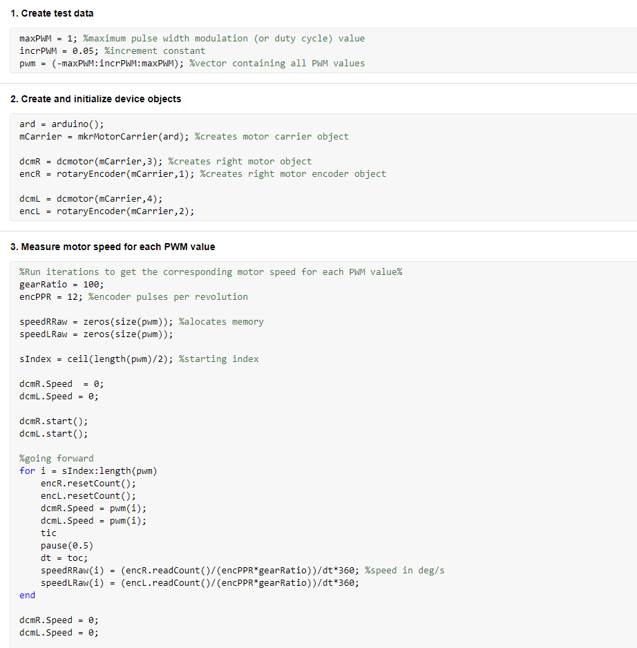
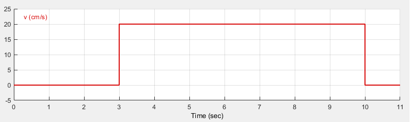
This is the basic algorithm: first, we have the input speeds, which now are signals that change over time instead of fixed numbers:

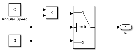
Then, we have the kinematics block, which is the same one as before. Next, we have the encoder simulation, which is a simple derivative of the speeds that as a result gives us the angular displacement in degrees (in the real model, the encoder will give us the number of pulses, from which we will calculate the angular displacement, but here we chose to simplify it since it will not change anything):

distance calculation

angle calculation


X and Y calculation

path plotter


Here is the result of this simulation:


Note: when using an Arduino board, we cannot really change the supply voltage in an analog way. Instead, it uses a technique called PWM (pulse width modulation) to have the same effect when working with digital signals. You can learn more about it
With this, we can now proceed to implement the model on the real robot. The Simulink model will be similar to the simulation one, but now we will feed the desired angular speeds to a lookup table with the motor characterization data, which will perform interpolation and give the corresponding voltage. We then feed this to the motors:

left motor

right motor


By changing the value of the integral gain, we can also change the motor's acceleration, so instead of instantly going to the desired speed, as before, now it can reach it gradually. Let us see how it performs with 3 different gain values:
As we can see it performs quite well. Below are the images of the signals for a better comparison:


left motor controller

right motor controller

speed inputs


linear speed


angular speed
dashboard controller

This controller allows us to move the robot around and also adjust its speeds using the knobs. Let us see the simulation:
Now we will add the controller to the model that we run on the real robot. Other than the previous movement commands, we will also add a new one to lift and lower the forklift:
8. Conclusion
In this chapter, we saw how to obtain the robot's equation of motion in order to get a transfer function and how to implement it on a Simulink model to move it both in a simulation and in the real world. So far, what we are doing is called forward kinematics, which is basically when we directly drive the robot the way we want to and make it go to a certain location. Next, we will develop new algorithms to do the opposite: we will give the robot the trajectory it should follow and it will drive through this path. This is called inverse kinematics.
1. Introduction
In the previous chapter, we controlled the robot by selecting the percentage of the total voltage that we would feed to the motors. The numerical values we used ranged from -1 (-100%) to 1 (100%). It is important to notice though, that these are not the actual voltage input, but were chosen to simplify the understanding. With this robot, we are using a 3 cell lipo battery, each with a nominal voltage of 3.7V. Therefore, our battery provides a total of 11.1V to the dc motors.
Intuitively, we know that if we feed a low voltage to the motors, let us say 0.2 (20%), the robot will drive slow, and if we provide a high value, such as 0.9 (90%), it will drive much faster. We do not know, however, its actual linear or angular speed.
In order to know the robot's speeds at any given moment, we will have to derive its equations of motion and manipulate them to a final form where for given inputs (in this case the wheels' angular speeds) we can calculate the respective outputs (in this case the robot's linear and angular speed) and vice-versa.
In control theory this equation is called the "transfer function" of the system. It is important to realize that the chosen variables are arbitrary and are selected based on the problem that we are trying to solve. For this one in particular, it is convenient to choose the wheels' speeds and the robot's linear and angular speed as the variables, since whenever we talk about a vehicle, the first thing that intuitively comes to mind in order to understand its functioning is its speed.
2. Obtaining the equations of motion
Let us begin by analyzing the diagram below with the robot's speed and dimensions and determining what are the equations that define its movement:


left wheel
right wheel
Our robot has two speed components when it is moving at any given time: the linear speed V and the angular speed W. These speeds are a result of the combination of the angular speed of the left and right wheel, wl and wr respectively. The wheels also have their linear speed component, vl and vr. Lastly, R is the radius of rotation of the robot, and cr represents the center of rotation.
Regarding the dimensions, we will call L the distance between the wheels, and r the radius of each wheel. For this one in particular, L = 8.8cm and r = 4.5cm.
Now we can begin writing the equations of motion:
(1)

(2)

(3)
(4)

(5)

After combining the equations (2) and (4) for the left wheel, and the equations (3) and (5) for the right wheel, we can manipulate them to get the following:


We can then write these two equations in a matrix form in order to simplify it:

This is the final kinematic equation that we will use throughout the entire project. We can see that it is now in the format we wanted: the only variables are the robot's linear and angular speed, and the angular speed of the wheels.
With this equation, we can easily calculate how fast the robot is moving by knowing the angular speed of each wheel, which we can do by reading the encoders' pulses. On the other hand, if we want the robot to drive at specific speeds, we can calculate exactly at which speed each wheel has to rotate in order for it to do so.
It is also important to notice that we manipulated the equations in order to eliminate the variable R. If, however, by any reason we thought that it would be more interesting or intuitive to use the radius of rotation of the robot instead of its angular speed, we could have done so too. In this case, we would eliminate the variable W and would have a slightly different final equation.
3. Basic kinematics with Simulink
Now that we have the governing equation of the robot, we will begin to build the model in Simulink in order to simulate its behavior and then upload the algorithm to the real thing.
First we insert the kinematic equation as below, then, we transform it in a subsystem so that it is simple to understand and reuse later. Note that the units chosen for the linear speed are centimeters per second, and for the angular speed degrees per second.

4. Calculating the robot's position

One way to find the robot's coordinates and heading would be to calculate its linear and angular speed and then integrate them:


To do so we would use the encoders to find wl and wr and then calculate V and W using the equations of motion in section (1).
This is not, however, the best approach. Since the rawest value that we can compute is the angular displacement of each wheel, we can derive new equations to calculate the robot's position and direction using them directly instead of using them to find the angular speed of the wheels, then using these angular speeds to find the robot's speeds, and then finally integrating these to find its displacement.
If we write the equations (1) - (5) in section 1 in terms of displacement, instead of speed, we find:
(5)

(6)
(7)

(8)

(9)
Where sl and sr are the left and right wheel linear displacements.
In order to really understand how we are going to obtain the robot's position and heading, first we have to realize that what we are going to do is not directly calculate it using a formula, the way we did with its speed. Because the robot's coordinates are based on a frame of reference, we will start from a known position and direction (x0, y0, theta0), and from there we are going to calculate how much the robot has traveled at every few milliseconds and add it to the previous position value.
These milliseconds are called our sample time, during which the wheel speeds remain constant. Since we are implementing a discrete model, we will choose our sample time, which for this project will be 10 ms. If we were building a continuous model, then this "sample time" during which the speeds are constant would be infinitely small, tending to zero, and usually represented by dt.
By combining the equations (6) and (8), and the equations (7) and (9), we will obtain two new equations. By subtracting the second one from the first one, we will get:

This is how much the heading will change at every sample time, considering that the value of the wheels' displacements are reset to zero in every new iteration. That is why we added the dt symbol to theta. We need to keep adding all these values together in order to get the current heading:

As we can see, the only variables that are in the sum are the wheels' displacement, which we calculate using the encoders' pulses. The encoders, however, already give us the full summation. They do not reset the count at every sample time. Because of this, we will not have to add the values together again in our simulation, and so the final equation that we will use in the algorithm becomes:

To find the position in X and Y coordinates, we can combine the equations (5), (8), and (9) to get a new equation with s, sl and sr only. Then, if we replace this new equation in equations (6) and (7) we will find:

Again, this represents the robot's total linear displacement during each sample time, considering the angular displacements of the wheels are reset to zero at every iteration. To know the total displacement, we will have to add them together:

If we only wanted to know the robot's total linear displacement, that is, the total distance it has traveled, we could use the same logic of the angular displacement, that the encoders give us the total sum of the pulses with which we obtain the total sum of the displacements and therefore we can remove it from the algorithm.
In this case, however, this is not valid anymore. Here, we must know the distance the robot has traveled only during that specific time sample. By combining this information with its heading angle, which is constant during each iteration, we can calculate how much it moved in each direction, X and Y. If we only had the total linear displacement, it would be impossible to know its location, since it can travel a specific distance by going through pretty much any trajectory (straight line, zig-zag, circles, etc).
By decomposing its sample time linear displacement into X and Y components, we find the final equations that we will use:


Now that we have all the three equations we need, we develop the model on Simulink:

Lastly, we have the position calculation subsystem, which implements equations we derived earlier and also a Matlab function that will plot the robot's position:
...
5. Running the real model
Now that we've run the simulation, it is time to test it on the real robot. To do that, first we have to get the characterization curve of our motors. What our transfer function does, is tell us the angular speed that each wheel has to turn in order for the robot to move with a determined linear and angular speed. However, we do not know yet the exact voltage supply each motor need in order for the wheels to turn at those speeds. To know that, we are going to "characterize" the motors. That is, get a voltage x wheel speed relation.
Basically, we are going to make the robot drive forward and backward with different voltage supply values and get the corresponding motor speed for each one of them. Next, we manipulate the results in order to remove non-increasing values, since each speed can only have one corresponding voltage, and finally, we make sure that zero voltage corresponds to zero speed.
To do that, we will write a live script using Matlab, so that we can run it whenever we want:
We can see results on the plots below. The blue line is the raw data, and the orange one is the data after we manipulated it in order to solve the issues mentioned in the beginning of the section.
Let us try the same speed inputs as before with the simulation and see how it goes:
As you can see, it does not perform exactly how it was supposed to. This is due to the fact that our characterization procedure was very simple. We only drove in a straight line, without considering other cases, such as when it turns a lot or a little in both directions and when it has to turn in place or using only one wheel. All these other cases may require more or less voltage in order for each wheel to turn at the same speed. Moreover, even if we do get a very strict and precise characterization curve, changes in the environment such as a different surface type or angle will require a new procedure for it to do well. Other factors, such as a different battery level will also compromise the current data. These issues are all characteristics of open-loop control. Open-loop control is only desirable when our model and the environment it will work in will not change.
Next, we will add closed-loop speed control to the motors to tackle this issue and also introduce a new feature: acceleration.
6. Closed-loop speed control
Our model will be a simple integral controller that will read the desired and the current speed and increase/decrease the motor speed based on the error between the two until it reaches the desired one.
We also need to add a reset in order to bring the integral value back to zero when the motor stops. Otherwise, because of the fact that at very low voltages the motor does not turn due to its inertia, when we change the rotation direction it will take a while to start turning since it will not be starting from zero, but from a small voltage value in the other direction where the motor first stopped:
We can notice that there is a small delay before the motor starts turning when it is starting from zero speed. This is due to its inertia, as mentioned before. The controller begins to increase the supply voltage but the motor only starts to move when it reaches a certain value.
Now, let us add this new speed controller to the previous Simulink model and see how the robot moves. First we have to run a new simulation model with the controllers added:
Let us run the simulation:
Now we will add the speed controllers to the model that we run on the robot so that we can compare the expected and the real results:

left motor controller

right motor controller

left motor

right motor
And finally, we can see how the real thing performs using the same speed inputs as before:
Note: the arena in the simulation has the same size as the real one (140x100cm), and so does the robot.
This time, with the speed controller, it really moves the way it should. This is a better approach than the motor characterization we tried before because it does not matter if the surface roughness is different, if it is downhill or uphill, or if the battery level is not full. The controller makes sure that the wheels always turn at the desired speed.
7. Controlling the robot through Wi-Fi
So far when moving the robot on the arena, we used signal builders to set its linear and angular speeds over time. In this section, we will build a kind of a virtual remote control on Simulink so that we can play around with it.
The model will basically be the same, except that now the input speeds will be given by the controller that we will add:

lift rate

dashboard controller

Here is how it works:
DIFFERENTIAL DRIVE ROVER: PART II