distance = 20cm
distance = 1.5cm
From the figures, it becomes clear that long distances will make the robot deviate from the desired path, while too short distances will cause it to oscillate and eventually become unstable. This instability didn't happen on our simulation, but if we lowered the distance even more it would.
8. Conclusion
In this chapter, we saw how to develop inverse kinematics by using closed-loop to control the robot's linear and angular displacement. We then developed three path-following algorithms using them. Each one of these has its uses, depending on the task that we want the robot to perform. Differential drive robots have many uses, from cleaning robots that wander around the house to shelf-carrying robots that work in modern warehouses, such as the ones from Amazon. The algorithms in this chapter could serve as a basis to develop more complex ones suited to the particular needs of the industry.
So far, we have only done open-loop control regarding the robot's position, since we specify the desired speeds and have no way to make sure it is moving where we want it to. For example, if we wanted it to drive 100cm forward, stop, and then make a 90° left turn in place, we could set its linear speed to 25cm/s for 4 seconds, while the angular speed is set to 0, and then set the linear speed to 0 and the angular speed to 45 deg/s for 2 seconds. This is assuming instant speed response from the motors. If we use acceleration, it becomes more difficult.
This way of displacement is not precise and is also subjected to outside factors that could change the robot's trajectory and we wouldn't know since we have no feedback on its location and heading. A good example would be an obstacle on the ground that changes its direction or block its passage.
In this chapter, we will add closed-loop control to the positioning. This will allow us to develop its inverse kinematics. First, we will create PID controllers for the linear and angular displacements, and then we will implement three different trajectory algorithms to drive the robot.
Before we develop the path following algorithms, we have to make sure the controllers we are going to use with them are accurate and tuned to our particular model and results that we are trying to achieve.
We will begin by implementing a linear distance PID controller to our previous Simulink model. As we will realize, we will also need to add another controller for it to drive straight. The new blocks are marked in blue on the model. All the rest remains the same as before:

(click on the image to enlarge)
linear distance controller


drive straight controller


Let's understand a few simple things about this controller:
- The error we are measuring is the difference between the linear distance we want it to drive and the actual distance it has driven so far. This error is fed to the PI controller and the result then serves as the input linear speed of the model. This will cause the robot to drive fast when it is far away from the location it should go to, and slow as it approaches it.
- Because we have acceleration in our motor speed controller, we can also make it move slow in the beginning, when the controller output linear speed will be high, but the motor will have to accelerate in order to achieve it, instead of instantly going to that desired value.
- The switch on the linear distance controller makes sure there is no overshoot by turning it off (feeding zero) when the error is equal or less than zero. Because of this, there is no need for a derivative term, and we can only have a PI (proportional-integral) controller.
- The reset block does the same thing as before: it resets the integral when the error is zero.
- The setDirection function was created to make the robot turn in the shortest direction (clockwise or counterclockwise), depending on the error. For example, if its current heading is 30° and it hasto to turn to 350°, it won't turn 320° clockwise, but 40° counterclockwise instead.
- There is no need for the integral term on the drive straight controller due to its characteristics: the error is low, the gains consequently have to be high to make it respond fast, and it is constantly adjusting, which means it does not go to a steady state where there could be a steady-state error for the integral to correct.
Let's run the simulation with arbitrary gain values to show why we need the drive straight controller. In all simulations, we want the robot to drive 100cm straight. First, we will run one without, and then one with the controller:
As we can see, the greater the proportional gain (P), the faster the robot's speed is, especially in the beginning, where the error is high. If, however, we have no integral term (I), we have what's called steady-state error, which is when the robot has stopped moving, but hasn't yet arrived at the final location. We can notice this in the first case of the simulation, where it stops before reaching the 120 coordinate on the X axis. This happens because the proportional term has become so small that it can't overcome the robot's total inertia. In this case, we need to add an integral gain, which accumulates error over time and isn't only based on the current error, like the proportional one. In general, the greater the integral gain, the faster the robot will move when it's close to its destination. We can see this difference in cases 3 and 4 of the simulation, which have the same proportional gain, but one also has integral and the other doesn't.
Now let's test it on the real robot. Here's the Simulink model:

(click on the image to enlarge)
And here's the robot movement for different gain values. The black lines on the yellow stickers on the arena mark the 100cm distance that it should cover.
We notice the same thing that we did on the simulation regarding the robot's behavior: the proportional gain influences its general speed, and the integral gain how fast it moves when it's close to the destination, when the proportional gain is low. Of course the integral gain also influences the general speed of the robot, because it's integrating the error since the beginning, but it affects its behavior the most when close to the steady-state.
Here are the controller responses on the scope:

P = 0.2 I = 0.01

P = 0.4 I = 0.005

P = 0.4 I = 0.1

P = 0.9 I = 0.1

(click on the image to enlarge)
angular distance controller

We turn the controller off when the error is small than 0.1 to avoid overshoot. We are doing it this way instead of adding a derivative term because it will be more suitable when we use it in our path following algorithms.
turn in place controller

Similar to the drive straight controller, in this case we have a turn in place controller. Again, due to the fact that the motors are not perfectly equal, one may accelerate a little bit faster than the other and it can cause the robot to move, so we implement a controller to compensate for it.
Let's run a few simulations to see how it behaves with different gain values:
The controller works as expected. Now let's try it on the real model:

(click on the image to enlarge)
Here is the robot's response for different gain values when turning 90 degrees:
The controller does work fine and we will keep these gains in mind when implementing it on the trajectory algorithms. Let's also see their response on the scope:

P = 0.4 I = 0.005

P = 0.8 I = 0.1

P = 2.0 I = 0.2

P = 4.0 I = 0.5
The first thing we'll do regarding the path following algorithms is develop a Matlab function for us to choose the robot's path.
We'll create an empty graph matching the size of our physical arena, then click on it to define the points through which the robot will pass. After defining the points, we have two options: Simple mode will keep the same points we clicked as the points the robot will go to, while Full mode will interpolate the chosen points and create a trajectory function. Next, if we selected full mode, we'll choose the distance between each point on our trajectory, since the algorithms will work with points coordinates and not the function itself.
Here's our Matlab function:

simple mode

trajectory function
We get this function using Matlab's curve fitting tools. The chosen method was cubic interpolation, but we could also have chosen others, such as polynomial, linear fitting, gaussian, etc. Each one of them generates a slightly different curve.
If we choose the full mode and the distance between each point, then we get a new set of points that becomes the robot's trajectory. Below are two examples with different distance values:

full mode, distance: 10cm

full mode, distance: 2cm
Note that what matters in the end are the blue points, which will serve as "targets" for our path following algorithms. The red line is just the function through which they were generated, but it doesn't necessarily mean that it will be the exact robot's trajectory. That will depend on the algorithms and how well we will be able to implement them and tune the controllers.
5. Stop-and-Turn algorithm
The first algorithm that we'll implement is pretty self-explanatory. The robot will start at the first chosen coordinates and with a heading of zero degrees as default. It will then turn until it's facing the next point, and drive straight until it reaches it. It will repeat this logic until the last point.
To develop this and the next algorithms, we'll use a Simulink control tool called Stateflow. This will allows us to create a model using state machines and flow charts. We basically will develop loops, or "states", that will be run until a certain condition is met.
Just like before, the only thing that will change with our Simulink model is the speed inputs, that now will come from our Stateflow chart. The points that make up our trajectory are fed to it from the pointsCoords constant block.

(click on the image to enlarge)
Below is the Stateflow logic. Each block is a loop that is run until the condition inside the [ ] next to the arrow line is met. The code inside the { } is executed when the logic follows that path. The code after the entry: and exit: commands is executed only once when entering and exiting the block.


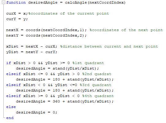
Inside the states, we use the Matlab functions calcDist and calcAngle to calculate the target distance and angle that the rover has to move in order to get to the desired location:
target distance calculation

target angle calculation
Then, we feed the outputs of these functions as inputs to the controllers, which are present on our Stateflow model as Simulink functions. These controllers are the exact same that we developed in the previous sections. There's only a small difference with the linear displacement control. Here, the error calculation (desired distance - actual distance) is done by the Matlab function calcDist, instead of by the controller, and directly given to it:
linear distance control

drive straight control

angular distance control

turn in place control

We'll begin by choosing a few points for the trajectory using the function we created, and then we'll select mode 1:

Now, let's run the simulation to see how it goes:
It works as expected. Let's implement it on the real model:

(click on the image to enlarge)
And here is how it performs:
We also added a XY graph block to the real model so that we can compare it with the simulation:

simulation

real
As we can see, the model that we've built is accurate. We could tune it further if we wanted it to work with very small linear and angular displacements, as the gains we are using right now maybe wouldn't be able to move the robot in those cases. Maybe we would have to add more logic to the algorithm in order for it to use different gains depending on the initial linear and angular distance between the current and the next point.
Another thing we could do is test different speed controller gains to reach desired acceleration/deceleration behaviors. If we use a high integral gain, the robot will start moving at max speed and slow it down as it reaches the location. If we use a low gain instead, it will accelerate in the beginning, reach the location at a high speed, and suddenly stop. If we want a mixed behavior, for example, for the robot to start moving slowly, then accelerate to a maximum speed, and then decelerate to slowly reach the target location, we will have to find a balance between the speed controller and the distance controllers gains, as we've mentioned before, in order to achieve it.
6. Move-and-Turn algorithm
The next algorithm will be similar to the previous one, but now, instead of stopping before turning, the robot will always be moving forward.
Here is the new Stateflow chart:

The two key parameters here are the values of the angular speed controller gains and of the distCdtn variable, which determines within which distance from the target point the robot will begin to turn to the next one. Changing these two values will impact the robot's trajectory, as we'll see later. The linear speed is constant.
The logic is simple: the robot will turn the first time towards the second point and will start moving forward. When it is within a certain distance (distCdtn) of its target point, it will begin to turn towards the next one until it's facing it. The loops then repeat until the last point is reached.
Let's run the simulation first:
We notice that in this case, the robot doesn't pass through the exact points coordinates. This is because we are using only one point for each curve. The only way it could make a good symmetrical turn with those points in the middle is if we added more of them.
Now let's see how the real model goes. The Stateflow chart is the same one used in the simulation:
Apparently it seems to be working as expect. We can compare the plots to see the trajectories:

simulation

real
The paths are very similar, with only a small difference in the angle of the second turn.
It would be interesting to show how the two main parameters can change the trajectory. Let's run a few more simulations with different values to see how it behaves:

short distance - low gain
long distance - low gain

short distance - high gain

long distance - high gain
The plots are pretty self-explanatory. The distance impacts how close to the points the robot turns, and the angular speed gains how fast, which results in a bigger radius.
As we've mentioned before, we could add more points to the curves to have more accurate turns. Here are the resulting trajectories with short and long distances. In this case, we can't play around that much with the angular speed gains because they need to be high enough for the robot to turn in time, since the points on the curves are close to each other:

short distance - high gains

long distance - high gains
One other thing we could do is create some sort of logic for the linear speed. So far it's constant throughout the drive, but we could, for example, use its controller to accelerate the robot when it's driving straight, and slow down before and while making the turns.
To conclude this section, this path-following model can be useful when we want the robot to pass through a few key coordinates while moving forward or avoid them by setting the distance value high. However, the general trajectory is still not very well defined and can change quite a lot for different gain/distance values, as we saw above. Next, we'll implement the final algorithm in which the robot will follow a well-specified path by us.
7. Continuous-Pursuit algorithm
Our final algorithm is called "continuous-pursuit" because the robot will always be chasing a waypoint that's ahead of it. We'll use the "full mode" of our path-defining function from the previous section to draw the trajectory.
Below is the new Simulink simulation model. The only thing that we've changed is the Stateflow block.

In the new Stateflow chart, we don't need the "driving straight" state. Now that the waypoints will be close to each other, the robot will always be turning. We've also removed the "turn in place" controller from the model to make it simpler, since the robot will only turn in place once in order to face its second waypoint before it starts driving forward. Let's see how the new chart looks:

The most important parameter here is the distance within which the robot starts pursuing the next target point. A long distance will cause the real trajectory to deviate from the desired one, and a too short distance will cause the robot to oscillate (overshoot) and eventually become unstable. That being said, it's not hard to find a value that will produce a trajectory like the one we want. The range between the "too long" and "too short" distances that don't work is big.
The angular speed controller gains also have to be higher here than on the previous algorithms because the robot has less time to turn due to the fact that the points are closer to each other. We had to tune the controller to reach the point where they are high enough for the robot to be able to perform close turns, but lower enough so that it doesn't do it too fast and overshoots. If we, for example, increased the linear speed, which now is set to 20cm/s, we probably would have to tune the controller to higher gains, since the current ones wouldn't be high enough for the robot to make those same close turns of before.
Let's begin by drawing a trajectory using the function that we've created before:

The blue circles on the graph above are the points that we chose. The red line is the function that was generated from them. Next, we have to choose the distance between each of the points that the robot will go to. Since this time we want it to be precise, let's choose a small value: 2cm. Here's the result:

This is the final trajectory that we want for the robot. Let's run the simulation to see how it performs:
It works quite well. The robot follows the full trajectory the way it's supposed to. The green circle shows which point the robot is pursuing at any given time. Now, let's try it on the real model:

(click on the image to enlarge)
The Stateflow chart is the same as in the simulation. Here's how it goes:
The robot is following the trajectory as intended. Let's also compare the simulation and the real path to see if there are differences:
simulation

real
The paths are pretty much the same, so we can conclude that our algorithm is working. Let's run a second simulation to see it working again. Here are the picked points and final trajectory, with 3cm distance between the points:

picket points

final trajectory
Here's the simulation:
And the real robot:
Finally, let's compare the two plots:

simulation

real
Our algorithm is working fine. The chosen pursuing distance is a good one that makes the robot precisely follow the desired trajectory.
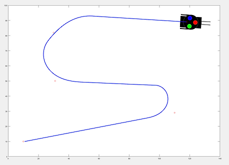
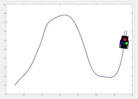
To finish, let's see what happens if we pick a distance that's too long or too shot. We'll run two simulations, the first with a distance of 20cm, and the second one with a distance of 1.5cm. You can check which point it's currently chasing by paying attention to the green circle along the path.
Let's take a look at the final trajectories:
1. Introduction
2. Linear displacement controller


without the controller
with the controller
From these images we can clearly see that without the controller the robot does not really drive straight. This is due to the fact that since the two motors are not perfectly equal, but the integral gain from the motor controller is the same, one of them will accelerate slightly faster than the other, causing the robot to turn a little. The difference becomes even greater if we use higher gains or acceleration. With the real model this becomes easier to notice.
Now that we know the drive straight controller is necessary, let's play around with the gains from the linear distance one to see how it works:
Note how there's no overshoot because we turn off the controller when we reach the desired target. Another point is that when considering the gain values that we are going to use with the algorithms, we also have to account for when the desired linear/angular displacement will be low. On the cases above, the error was high (100), and so were the controllers outputs, but what if we wanted the robot to move only 10cm? In this case, a low proportional gain would not be enough for it to start moving. So in the end, we will have to choose a gain that works with low and high distance displacements within the size of our arena.
Let's take a moment to analyze the behavior of some elements of the controller. First, let's see how the motor speed controller is working in the model. For this, we keep the linear distance controller gains the same, and run the real model with different integral gains for the speed controller. The results below are a plot of the desired motor speed x actual motor speed in deg/s:


As we can see, the controller is always "chasing" the desired speed, and the higher the gain, the faster it gets there. However, this also means a higher speed towards the end, when the robot is getting close to the desired location. To have a nice balance of acceleration in the beginning and deceleration in the end, we have to tune both the speed controller and the linear distance controller gains to this end.
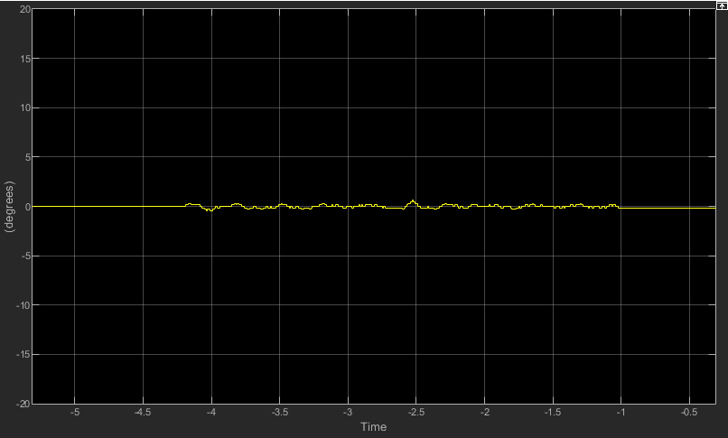
Next, let's take a look at the drive straight controller. Although it's not possible to use the simulation model plot when running the model on the real robot, we can add an "XY Graph" block to plot its position. First, we run the the model without the drive straight controller:

The first block is from the error scope. That is the difference between the desired angle and the real angle. We can see that without the controller, the robot's heading changed about 4 degrees over time. Below is the xy plot. We can see that in fact, the robot didn't drive straight.

Now let's test the robot again, but this time with the drive straight controller on:

We can see that now the robot's direction isn't changing over time like before, but it's oscillating very close to zero. To get to this behavior, we had to tune the controller by testing different gain values until we found the ones that work for our model. A low P gain won't correct the error fast enough. A high P gain will, but it will overshoot constantly in both directions. By adding a derivative gain, we are able to reduce the overshoot significantly, up to a point where it's acceptable, since now when we look at the second figure, the robot is driving pretty straight. If we use a higher derivative gain though, trying to reduce it further, the robot becomes unstable.
3. Angular displacement controller
Now that we have our linear distance controller, let's implement the angular distance one. As before, most of the model will remain the same. The only blocks that will change are the ones of the controllers that serve as input to the robot's speeds and are circled in blue:
...
Now that we have the controllers we need, we'll develop the path following algorithms.
4. Defining the robot's path
Let's see how it works. First, we click on the empty graph to choose the points that we want:

If we choose the simple mode, it makes the points we clicked the robot's trajectory. In every case, it also shows the resulting trajectory function from the points.
DIFFERENTIAL DRIVE ROVER: PART III


