


...
...

(click on the image to enlarge)
We've also created a new Stateflow logic for this task. The controllers remain the same:
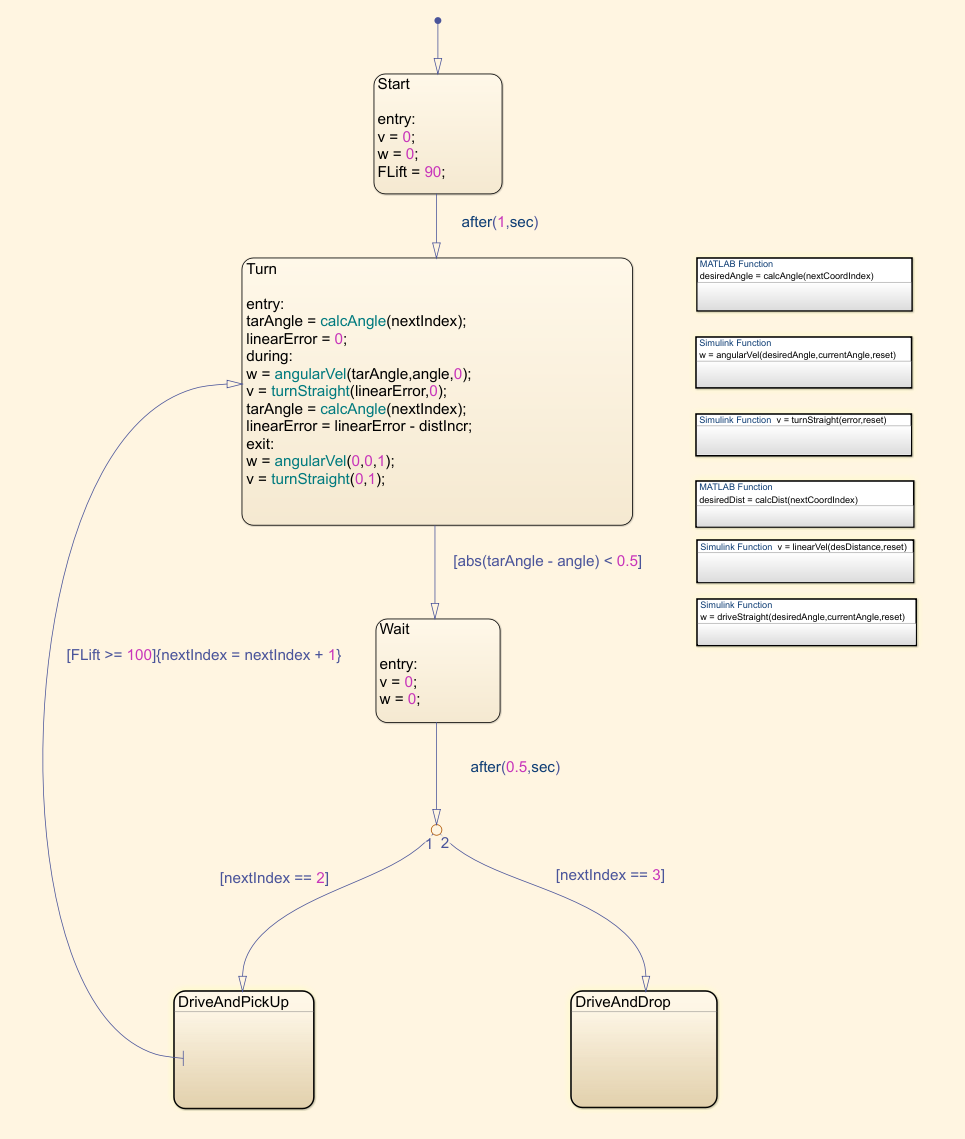
drive and pick up

drive and drop

Since now the coordinates we have are the points where we pick up and drop the target, and not the robot's locations like before, we have to make it stop before actually reaching the desired waypoints to account for the fact that the target is a few centimeters in front of the robot.
Here's the snapshot we took again:

And now let's see how the model performs. As we can see on the image of the Simulink model, we've added a third waypoint to the matrix, which is where we want the robot to drop the target.
It really does work as expected, so we can conclude that our algorithm is working and that our image processing is accurate.
(click on the image to enlarge)
Here's the new components that we are going to use:

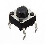
The joystick has five pins, two for feeding (+5V and ground) and the three outputs that we can read: X, Y, and button click, which we won't be using this time. It basically works like a potentiometer and gives us a voltage value. Therefore, we'll be using the analog pins on the Arduino to read it. The Arduino Uno in particular measures this data as a 10-bit value, meaning the range will be from 0 to 1023. So for example, when the joystick is standing still, we'll get an output value of about 512 from both directions, and if we press it fully forward, we'll get 1023 for the Y and 512 for the X direction.
We'll be limiting the maximum linear speed to ±50 cm/s and the angular speed to ±720 deg/s. To do this, we use two lookup tables that will convert the joystick reading to this range. Since we've adopted the counterclockwise direction as positive, we also have to change the signal of the X direction input, or it will turn right when we push the joystick left.
The two buttons are simple switches, and will be connected to digital pins on the board. For some reason, we are getting an oscillating signal when it's not being pressed. This isn't because the pin is floating when not active, as we tested it with a resistor and got the same results. On the Arduino IDE it works as intended but on Simulink we have this problem. To solve it, we added a function to clean the signal. It checks if the signal was zero on the previous 3 sample times, and if so, outputs 0. Otherwise it outputs 1. Here's the reading without and with the clean signal function:

And here's the function itself:


Regarding the motors, now we'll use the data from the characterization we did earlier to drive them. This is because the speed controller we created before was on Simulink, and the code we're going to write to run the board now will be on the Arduino IDE and we don't want to write a new speed controller code at this time. Also, on the new IDE the motor duty value goes from -100 to 100, and not from -255 to 255 (1 byte) as before. That's why we're multiplying the output of the lookup table by a different value:
left motor

right motor

Lastly, we'll send the outputs: left motor command, right motor command, lift on/off and lower on/off to the board on the robot using TCP/IP communication. That board we'll be the server, and the one connected to Simulink we'll be the client. We pack the signals of the motor and the forklift together so that we only use two ports. Also, because the data is sent in 1 byte packs, we have to convert it to int8 using the data type conversion block.
The Simulink model for the One board is ready. Now we have to write the code for the MKR1000 board that we're using on the robot. We could've done this by creating a new Simulink model for it, but we wanted to do it programmatically using the Arduino IDE to show how it works. Here's our code:

Now, let's run the model and play around with the robot on the arena:
The joystick gives us a lot of freedom on how to drive it. We can control the linear and angular speeds independently in an easy way. We can, for example, have a slow angular and a fast linear speed, or vice-versa. We can also change them very quickly if we so desire. The object that we have is a little difficult to pick up, since it will fall to the sides if the forklift isn't very close to the middle, but we can have fun with it nonetheless.
6. Conclusion
With this, we finish the differential drive robot. Even though it's a cheap project to build, we were able to cover some good engineering concepts and techniques and saw them implemented in the real world. They include:
- How to interface hardware, such as DC motors and servos with software (Matlab, Simulink, and Arduino IDE).
- How to obtain the kinematic equations of a system and manipulate them to give us a final equation we use to control its behavior in a discrete model.
- Open-loop and closed-loop control (DC motor speed control, linear and angular distance control).
- How to use Matlab to obtain and analyze data, interface it with Simulink, use it to plot simulations, and how to build functions, especially a path-planning function for a vehicle.
- How to build mechatronic models on Simulink using its various available blocks and how we use derivatives and integrals to calculate speed and distance traveled.
- PID controllers, tuning, and troubleshooting.
- Image processing with Matlab: geometric transformations, morphological operations, structuring elements, thresholding, and how to use them with a webcam and a robot to obtain its coordinates and heading.
- How to use Stateflow in Simulink models to create path-following and pick up/drop down algorithms.
- How to directly drive a robot through WiFi, using both a digital interface on Simulink and real hardware (joystick and buttons) with TCP/IP communication.
- How to write C++ code using the Arduino IDE to receive data through TCP/IP and drive a robot.
We could further develop this project to include more elements or more complex algorithms. For example, we could use the ultrasonic sensor we have attached to it to drive around obstacles or make it stop to avoid a collision. We could add a buzzer to be able to honk. We could create an algorithm to take a snapshot of the arena, let the user click on a point of the image, and make the robot drive to that location. We could use the attached IMU to get the robot's position and velocity so that we have a second source of data to compare against the encoder data. This would be a good practice since in some cases, if the wheels slip or the encoder signal gets noisy, for example, we would have problems. We could also be constantly taking snapshots and analyzing them for the same purpose.
There are a lot of possibilities on what to add to the project, but for now, we'll leave it like this. We hope to develop other rovers, such as a four-wheeled one, and then maybe we'll use some of these ideas.
DIFFERENTIAL DRIVE ROVER: PART IV
1. Introduction
In the previous sections, we defined the starting coordinates and heading for the robot, placed it in that position on the arena, and from there, once it started moving, we calculated its positioning using data from the encoders and a mathematical model.
In this part, we will use a webcam to take pictures of the arena with the robot, and through image processing, we will be able to determine the robot's positioning and heading. We will also add an object for the robot to lift and get its coordinates the same way. Then, we will create a new model to calculate the robot's and the target positions, drive the robot there, lift the target, and drop it in a final location.
To finish, we will use a joystick and two buttons to drive the robot on the arena and operate the forklift wirelessly using TCP/IP communication. To do this, we'll need another board to communicate with Simulink and the hardware, since our previous board will be on the robot.
2. Calibrating the model
We'll begin with image processing. Before we can calculate positioning from a taken snapshot, we have to calibrate our model to account for our lighting conditions and the fact that our view is a perspective. Since we are not looking at the arena from above, we need to transform the original image to make it look like it, so that we can correctly calculate the robot's and the target's location. To do this, we get the coordinates of the four corners of the arena and use them to perform a geometric transformation:
Next, we place the robot on the four sides of the arena and take more snapshots. We'll use these to account for the angle distortion mentioned before so that we can accurately calculate its position.


By applying the previous geometric transformation to the images, we can undistort the pictures:


We do the same for the target:


And get the corrected images:


You can notice from the crosshair that we have the user-click function ginput active on the top-view images above. We wrote the function below where the user clicks on the coordinates where the robot and the target were actually placed, and then clicks on their centers on the image. With these two sets of coordinates, we can calibrate for their horizontal and vertical location offsets. The im2orthoview function in the beginning undistorts the original snapshots using the first function we created.
To finish the calibration, we get the color threshold of the circles on top of our robot. The result is a matrix with the RGB values of each clicked pixel. We'll use these later as a sort of filter to remove everything else from the image. By doing this to all three circles and then getting their centroids, we'll be able to calculate the robot's location and heading on the arena.


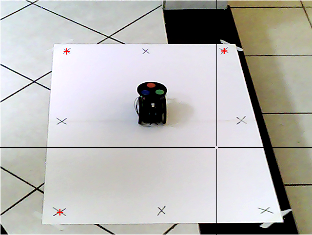
3. Locating the robot and the target
Now that we've calibrated our model to the environment's lighting conditions and camera angle, we can begin to process the image we take of the arena with the robot and the target in order to calculate their position. First, we place them where we want and take a snapshot. Them, using the same geometric transformation at the beginning of this page we transform the perspective view to a top one:
To determine the robot's coordinates and heading, we wrote the function below. It filters the image using the RGB values from the colored circles that we got before. This gives us three new black and white pictures where the only present form is the circle of that specific color:

red threshold

green threshold

blue threshold
Then, using the imopen and imclose functions from the image processing library and a structuring circle element, we get rid of points that do not have a radius of 3 pixels. This removes internal background spots and external small white spots so that as a final result we get only a good fully filled white circle:

final red circle

final green circle

final blue circle
To finish, we use the regionprops function to get the centroid coordinates of each of the circles. The center of these three coordinates gives us the actual robot's position.
To get the heading, we assume that the three circles' centroids form an equilateral triangle, with the red one pointing forward, and calculate its angle.

The next step is to calculate the target's coordinates. We do this in the same way we did with the robot. Except that now we'll be using only black and white thresholds and not colored ones.
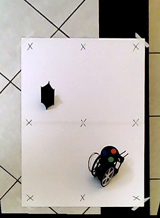
First, we crop the image using the marked corners to remove undesired black areas from it, leaving only the robot and the target:
Then, we threshold the cropped snapshot to black and white:
Using the same previous image processing functions, but this time with a 20 pixel square as structuring element, we remove the robot and other undesired points from the image:

We then get the centroid of the remaining element, the target, and add a constant to the coordinates to compensate for the cropping. Here is the function we used to do it:

Finally, with both the target's and robot's coordinates and heading, we also plot them on the undistorted image to have a visual representation.
Here's the full script that we used to perform the positioning calculation:
In the next section, we will use these results to drive the robot to the target, pick it up, drive to another waypoint, and drop it down.
4. Picking up and moving the target
Now that we can get the starting coordinates using the image processing algorithm, we'll create a new Simulink model using them as our waypoints. We'll add the servo motor to the model this time, since we'll use it to lift and lower the target, and also a third waypoint (xEnd, yEnd) to the matrix, which is the location where we want to drop off the target.
5. Driving with a joystick using TCP/IP
The last thing we'll do with this robot is move it around using a joystick. To do this, we'll need another board, which will be an Arduino Uno. We'll also add two buttons to lift and lower the forklift. The joystick and buttons we'll be connected to this second board, which will communicate through serial with Simulink, and Simulink will communicate with the board on the robot through WiFi:
First, let's take a look at the Simulink model. This time, it'll be a bit different from before. The inputs linear and angular speed we'll be the readings from the joystick, with V (cm/s) being the Y direction and W (deg/s) the X direction data.

In short, this algorithm creates a WiFi server connection with ports 80 and 81 and keeps reading the data sent from them. These are obviously the same ports on our Simulink model, with port 80 being the one for the motors' duty values, and the 81 for lift/lower values. These values are then used by the motor carrier to drive the DC motors and the servo.
As we've said before, the board on the robot is acting as the server, and the one with Simulink has the two clients, carrying the motors and lift data. Basically, the server.available() function gets a client that is connected to that server and has data available for reading. If no client has data available for reading, it returns false. Then, the client.read() function gets the data that was sent from Simulink to that particular server.
The most important part as to how the code works is understanding that multiple data sent through the same port is sent sequentially, one byte at a time. In Simulink, we coupled the data from the motors and the buttons using a Mux block before sending them, so that we only use two ports, instead of four. Taking the motors data as an example, this means that the first data that will be sent through that server is the one for the left motor. Next, the one for the right motor will be sent, and then the one for the left motor again, and it keeps alternating like this indefinitely. For this reason, we have the flagMotor variable, that we keep alternating between true and false using if statements in order to attribute the correct left or right motor data to its variable. The same logic applies to the lift/lower system.
Another thing worth mentioning is that we've also added some logic to remove unwanted noise from the motors signals. We're always reading the data sent from the joystick, even when it's not being pushed in any direction. However, we don't want to keep writing to the motor when the robot is standing still, so we send the command only one time for it to stop, and then send no more commands until the joystick is pushed again.
Here's a photo of our simple setup:


