DRAWING ROBOT:
PART III
1. Introduction
In this part, we'll process images to turn them into contour segments. This can be tricky since there are many possible cases for error, such as not being able to precisely extract only the drawing from the original image, getting a trace that's thicker than 1-pixel, which is the representation of a line that we want, or generating duplicate coordinates in the process. Once we have the pixel coordinates of the object that we want to draw, we have to order them into connected line trace segments so that the robot can draw the points sequentially. We also have to account for different types of images, such as line traces and full-painted ones. Lastly, we'll put all the workflow into an app that we'll make it easier to open, loop through the processing operations, and export the final result to Matlab's workspace to be used.
2. Turning regular images into line traces images
Matlab has an image processing toolbox with many functions that allow us to manipulate them. We'll write a live script to perform the task of converting a desired image to real-world coordinates to be drawn on the whiteboard. We begin by loading the original image:


Next, we'll use a few of the library functions to reduce it to line traces. Our goal here is to convert it to a binary image so that we can better manipulate it. To do that, first we convert it to a black and white (or grayscale) image:


Now it's easier to convert it to a binary image using a global threshold since each pixel only has one dimension, instead of three in the RGB one.


Note two things here. First, we got a nice image using the standard function parameters because this image is not hard to convert. In some cases, it might not be so easy and we may have to tweak the values of the function parameters such as the global threshold, or use the local "adaptive" threshold instead and change its "sensitivity" value in order to get a clean image. Second, we inverted the pixel values of the image using the "~" operator because in Matlab the background is represented by black (or 0s) and the image is represented by white (or 1s), which is the opposite case of our image, where our drawing is black.
After this procedure what we have is a binary image. We can now use tools to perform morphological operations on it. What we do next is remove any isolated pixel that might exist on the image. In this case they could be so small that we can't even see them, but they might be there nevertheless:


The final step is to thin the image until all that's left are its 1-pixel thin line traces:


By zooming in we can see that the lines really are 1-pixel thick, which is what we're aiming for. We only want the robot to draw one line for each trace.

3. Turning line traces images into coordinates
With an image that's made only of line traces, we can proceed to the next step, which is to get the coordinates of each point. To do that, we'll use a function that returns the coordinates of the boundaries of every object in an image.
An object is a group of pixels that is isolated, that is, not connected to anything else. They can be either connected lines, like roots, a closed-loop, or a combination of the two. In the case of a closed-loop, all the other lines inside of it are not considered objects themselves, but "holes" of its parent object, the loop.
We'll create our own recursive function to perform this task for us. We'll explain how it works, step-by-step, and then we'll show the whole code for it. First, we use the bwboundaries function to extract the coordinates of the boundaries of our image. In this case, we only have one object on the image. We also exclude repeated coordinates in case they exist and put them into a normal array, since the function returns them in a cell. Here's what we get:


Notice how the internal lines weren't extracted. That's because as we explained before, they are not considered boundaries of an object, but "holes" inside of it.
The next thing that we do is remove the extracted boundaries from the original image. To do that we perform a linear indexing. That is, we make all the coordinates that we extracted equal to zero. This is what is left:


Now, and this is the reason why this is a recursive function, we check if there is anything left on the original image, that is, if there are more lines whose coordinates need to be extracted, and we call the function again if that's the case:

When we call it the second time, the first boundaries that were extracted are not there anymore, so the bwboundaries function will get the next ones. In this case, the object will be all the lines that are left there, because there's no closed-loop. Here's what extracted:

Continuing, we remove those coordinates from the image as before, and here's what's left:

You can see that there's nothing else there. We've got all the images coordinates. So the condition won't be met and the function won't be called again.
When we plot the final array containing all the coordinates, we can see that we've really extracted the whole image:

Let's compare what we had before with what we have now to notice the difference:


Before, we have a binary image represented by a 480x640 pixel matrix. Now we have a 675x2 matrix containing only the coordinates of the foreground, or drawing pixels (white ones). Below you can see the whole function:

And our live script call:

4. Turning sets of coordinates into segments
So far what we have is an array with sets of coordinates. The next step is to turn these into segments. A segment is a connected set of waypoints that the robot will go through without raising the marker. We also wrote a function to perform this task. We won't be showing a visual representation of the steps because they are straightforward and easy to understand. Here's how it works:
Since all points in a segment are connected, the distance between each point in either the X or Y direction is 1. Therefore, the way we identify when a segment ends is by subtracting each coordinate by the previous one, and checking where this difference is bigger than 1. We call these discontinuities:

Next, we compute the number of discontinuities that we have. The number of segments will be this plus one. Then, we find the indices of these discontinuities and create an array with them that will be used to split our coordinates matrix:

Finally, using the discontinuities indices array, we split the original coordinates into segments:

Here's the whole function:

The call in our live script:

And the resulting image after the procedure, where each segment was plotted in one color:

Now that we have converted the coordinates to segments, we still have to perform some tasks to optimize them to be drawn. The next function that we've created will do two things: first, it will close gaps between self-intersecting segments. Second, it will merge segments that start or end where another begins or ends. This will become clear in the explanations that follow.
First, let's consider the case of self-intersecting segments. When we want to draw a segment that is a closed-loop, or that has a loop in it, we have to add an additional point at the beginning or at the end, or else we'll leave a gap there. For example, if we want to draw a circle, or the letter "P", on the left we have what will happen if we draw them as it is, and on the right how we can fix it by adding another point to the segment:
...
...
p3
p2
p1
...
pN
...
...
...
p4
...
p3
p2
...
p1, pN
...
...
...
...
p3
pN
...
p2
p1
p3, pN
pN-1
p2
p1
The normal robot's path will be to go from the first to the last point, but to close the gap we need one additional point because we also need it to go from the first/last to that adjacent point. This point will change from case to case. In our examples, it's the last point in the circle and the third point in the "P". Let's see how our function works:
Initially, we get the segment that we'll work on. First, we'll check for points adjacent to the beginning of the segment (first point) and then for points at the end (last point). We store its first point in a variable, and all but the first three points in an array. The reason we do this is to not repeat the procedure twice. When we do it for the last point, we'll include these.

Since we'll be doing this a lot, we wrote a sub-function to check if two points or a point and an array of points are adjacent. This sub-function verifies if both the X and Y coordinates of any of the points in the second array p2 is within a 1-pixel distance of the first point p1. This would mean that they are adjacents. It returns a row logical vector that indicates if that particular set of points is (1) or isn't (0) adjacent to the point with which it was compared:

In our main function, the next step is to call this function to verify if any of the points of the second array is adjacent with the first point:
If that's the case, we use the function find to get its indice and add it to the beginning of that segment (first we actually add it to the beginning of the array "points", as you can see below, but at the end of the loop the array "points" become the segment):

Then, we use the same logic, but for the last point of the segment instead of the first. This time we include the first three points that were neglected the first time, and remove the last three ones, that were already verified. The logic is the same as explained before: to not do the same thing twice:

Let's move on to the second task: merge segments that are adjacent to each other. Due to the way that the coordinates were retrieved using the bwboundaries function, it could happen that we have two segments that basically could be the same, because one begins right beside the point where another ends, or vice-versa. In fact, if you check the last plot of our image, you'll notice that's exactly the case. Especially in the upper part of the image, on the hat, we have many segments that could be merged into just one. Here's what we're doing:
a1
aN
b1
bN
a1
aN
We've also written a function to perform this task. This one has more lines of codes but is actually simpler than the previous one. What we do is compare the first and last points of every segment and see if they are adjacent. If so, we add one segment to the beginning or to the end of the other and then empty it. Those two segments then have become one. To check if the points are adjacent, we use the same sub-function as before:

Here's the uninterrupted function:


And the call in our live script with the result:


Let's compare before and after. Notice how the green and the blue segments on the first image were merged together on the second:


To finish, we store the X and Y pixel range by getting the minimum and maximum values of each direction. We'll need these later to scale the image to fit in our whiteboard.

And here's how the final live script looks like:


5. Processing other image types
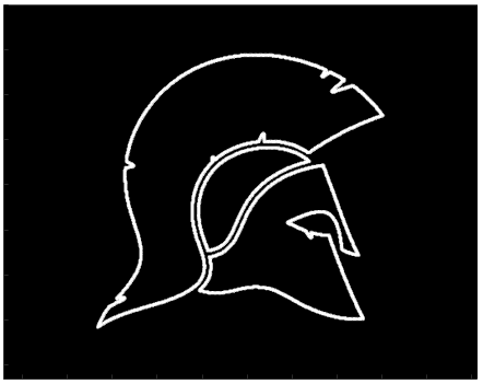
With the code that we've developed so far, we're able to draw images that are made of line traces and that also may have traces inside of them. But what if we wanted to draw full vector images like the one below?

In that case, we need to modify the function that first gets the image boundaries. Our current function is a recursive one. We call it multiple times because we want to get all the traces that may be inside of the image as well. However, in the case of full images, there are no traces to be extracted inside of them, only "holes" that are extracted in the same function call as the boundaries. Because of that, we only need to call that function once, so our modified function becomes:

Another thing that changes is that we don't have to perform the morphological operation "thin" on the image, since we don't have to thin any line traces. The boundaries that we extract are already 1-pixel thick. All the rest stays the same. Here's the full result for this particular image following the same order of the live script:
grayscale

binary

clear from isolated pixels

coordinates
segments

closed and merged segments

6. Building an app to process images
Since we may have to try different values for the threshold before getting a clean image when we transform it from grayscale to binary, it's useful to have an app that makes it easy to do. Moreover, an app helps visualize all the processes that the image goes through and is more intuitive than a live script.
We've built an app to allow the user to open images, process them, and export the coordinates of the final segments to Matlab's workspace. Here's its interface:

The user can open an image by searching folders, and then go through all the processes by clicking the buttons. The image type must be selected in the beginning. If the auto threshold doesn't produce a good result, the user can switch to manual and use the slider to find a value that gives a good and clean image. After the final step, when the segments are merged, the "Export" button is enabled and the coordinates can be exported to the workplace to be used by the drawing algorithm that we'll develop in the next part of the project.
Here's the app code:


Let's process a few images in the video below to see how the app works:
Notice how with the image "HELLO" we get an isolated coordinate at the upper left trace of the "H" letter and we go back and change the threshold to solve the issue. We also had to adjust the mountain image. The first time we choose a threshold value that's too low and creates many small segments on the right side. Then by increasing it a bit we get a better clean image with just three segments.
7. Conclusion
Processing an image to be drawn by our algorithm isn't so easy as it seems at first. We have to go through many steps to convert an image into 1-pixel ideal segments made of sequential coordinates that accurately represent the image's line traces. Now, however, we're ready to do that which was the main goal of the project from the beginning: draw it on the board. On the next and final part of the project, we'll put together everything that we've built to go from the process of obtaining an image to doing that, and we'll also add one more feature to allow the user to instantly capture an image that he wants to draw using a webcam.