ROBOT ARM: PART I
1. Introduction
In this project, we'll model and program a 4-DoF (degrees of freedom) robot arm that we can move in space, pick and drop objects, and follow desired trajectories:

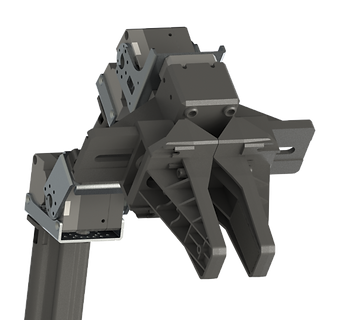
To move the robot we'll use 4 servo motors, acting as revolute joints. We can better see them in the image below, where the motor covers have been removed:

servo 1
servo 2
servo 3
servo 4
joint 2
joint 3
joint 4
joint 1
A fifth servo is used to open and close the gripper mechanism:

servo 5
open gripper
closed gripper
2. Multibody model
To simulate and visualize the robot's behavior, we will build a multibody model using Simscape. By using the 3D files, the materials data, and how the parts are connected, we have a system response that will be very close to the real-world model.
To begin we build the general model and test the movement of each joint to make sure it is working as intended. Here is the visualization of the multibody model that we have created with Simscape:

And here is the model:

base

servo1

servo2

servo3

servo4

servo5

gripper

To set the servos' position, we have added sliders that the user can interact with:

The manipulator outputs the current joint angles that we are going to use in the next step. For now, let us see if the model works:
The model is working as it should. We can tell by the movement that the connections are right and the servos are commanding the motion that we expect on each joint, including the gripper's.
3. Forward Kinematics
The next natural question that arises when working with robot manipulators is the need to know the position and orientation of the end-effector. Given the current joint angles, where is it located in space relative to the base coordinate system? This is the basic forward kinematics problem.
We begin by defining a cartesian (XYZ) frame in space for each of the joints. This frame is always a right-handed one, with the axis of rotation being Z, and the link frames being X. After these two have been chosen, the Y-axis is automatically given by the right-hand rule. Here's how we chose to define the ones for our manipulator:

link frames (orthogonal view)

link lengths and distances (side view)
Two things are worth pointing out here. First, as shown in the first figure, the origin of frames {1} and {2} is the same. Second, the length of the second link (a2) is not the vertical distance from frame {2} to {3}, but the distance between the two axes of rotation, Z2 and Z3. These frames have been defined following the Denavit–Hartenberg convention so that later we can easily compute the transformations from one frame to another. It is also important to notice that although we are free to position the frames as we please as long as we respect the D-H convention, we should try to choose the positions in a way that as many frames as possible have the same origin or have axes that are collinear, parallels, or orthogonal. This will greatly reduce the number of equations in the future, making both the forward and inverse kinematics problems much easier to solve. Consequently, this will reduce the number of computations necessary to find the solution, decreasing the need for a fast processor and lowering overall power consumption.
Next, let us see the robot in a different configuration in which it is easier to visualize the joint angles and how they are measured. The dotted lines are the projection of the respective axis to facilitate the visualization:

first joint angle (orthogonal view)

other joint angles (side view)
The convention here is that the angles are measured from the previous to the current X direction, and around the current rotation axis Z. So for instance, θ2 is measured from X1 to X2, rotating about Z2.
Then again, following the Denavit–Hartenberg convention we have the following parameters for each joint:

We are not going to go into detail here as to how the parameters of a robot manipulator are defined using the D-H convention or explain the theory behind transformation matrices. If you do not know that yet or you want to review it, please check our robotics learning section.
The transformation matrix from one frame to the next is the one below. It basically gives us the position and orientation of one frame in terms of the previous one:

With the system parameters from the table, we can find the transformation for each frame:

We can stack these transformations to get the position and orientation of frame {4} in terms of frame {0}:
At this point, you may be asking yourself why did we compute the transformation until frame {4}, and not until the end-effector, or tool frame {T}, which is what we really want to know? Usually, in robotics, we solve the general problems of forward and inverse kinematics from frame {0}, or base frame {B}, relative to the wrist frame {W}, which in our case is frame {4}. This is because the same robot may be used in different applications and therefore can have different tools. The end-effector of a welding tool will be different from the one of a gripper, which will be different from the one of a painting tool. In general, then, we solve the problem regarding the wrist frame and then make the final transformation to go from the wrist to the tool frame.
In this project, we are using a gripper. The end-effector location is in the middle of its fingers. From the way that we have defined its frame, its orientation will always be the same as the wrist frame {W}, or frame {4}, because they are attached to the same rigid link. Therefore, the only thing that we need to account for is the distance between the frames, or a translation, which in this case has the magnitude of along the X-axis. Hence, the transformation from the wrist frame to the tool frame will be given by the matrix:

Finally, we can compute the position and orientation, which we will call pose, of the tool frame in terms of the base frame:
or
To do this calculation we will write a script in Matlab, using the variables. It will then give us the final equation:

This yields a 4x4 matrix where the first three columns give the end-effector's orientation and the last one gives its position relative to the base frame. The last line is useless and is just used so that we can work with matrices and take advantage of known linear algebra operations:

Notice that regarding the orientation, what each of the columns gives is the projection of the tool frame onto the respective axis of the base frame.
Each of the matrix elements is a big equation involving sines and cosines. By using this notation:

And the identities below:

We can rewrite them in a more concise way. Starting with the position, the final XYZ coordinates are given by:
_PNG.png)
And for the orientation, we have for each axis:
_PNG.png)
_PNG.png)
_PNG.png)
Where:

4. Simulation
Now it is time to add the previous calculations to the model and simulate to see if they are correct. Our multibody model outputs the joint angles:

We feed the angles into a Matlab function to compute the previous equations:

And use a simple model that will show the pose in space, in the same environment as the robot:
pose representation

(click to enlarge)
In this model, a yellow ball will represent the end-effector's position. The XYZ axis will be represented by their standard colors: red, green, and blue, respectively.
Let's see the simulation:
By the fact that the position and orientation represented by the spheres correspond to the ones of the end-effector, we can confirm that our calculations and algorithms are working. What matters to us, of course, is the numerical value of the pose, which we can see in the display:

We will use these values given by the forward kinematics many times in future algorithms, whenever we want to know the current position and orientation of the tool.
4. Conclusion
In this chapter, we saw the basic mechanisms of the robot, built a multibody model, and solved the forward kinematics problem, which is, calculating the position and orientation of the end-effector for given joint angles. This is the most basic problem when it comes to robot arms. In the next part, we will solve the opposite: given a desired pose, what are the joint angles that will place the end-effector there? This is called the inverse kinematics problem and is much more complicated, as we will see.