ROBOT ARM: PART II
1. Introduction
In this chapter, we are going to solve the inverse kinematics problem. For a desired position, we are going to calculate the joint angles that put the robot's end-effector there. This is not as simple as it may seem, as other than calculating the solution (if one exists), we may have to account for other factors such as collision avoidance with the robot itself and other obstacles. Moreover, more than one solution can exist, and we'll have to design an algorithm to choose the one that fits our situation the best.
2. Workspace representation
When talking about solutions for the inverse kinematics problem, we have to check three things: if a solution exists, if there is more than one solution, and which method we are going to use to solve it. The question of whether any solution exists brings us the concept of the manipulator's workspace.
The workspace is the volume of space that the robot can reach. For a solution to exist, the desired location has to lie within the workspace. We may also divide the workspace into two categories: the dextrous workspace, which is the volume of space that the end-effector can reach with an arbitrary orientation; and the reachable workspace, which is the volume it can reach with at least one orientation.
In this particular project, because we'll always try to make the robot maintain a fixed orientation, we will only worry about the reachable workspace. Also, when talking about workspace, we always calculate it based on the wrist frame, not the tool frame, for the same reason mentioned before: the same robot may use different types of tools, which not always will have the same reference frame. With that in mind, we can see illustrated bellow how we are going to calculate the workspace for the wrist instead of the tool:

last frame: tool frame

last frame: wrist frame
If we consider the first joint to be fixed, our robot becomes a planar 2-link manipulator. It's intuitive to see that its workspace, obtained by rotating both the second and third joint to every possible position, will be a ring with an outer radius of a₂ + a₃ and an inner radius of |a₂ - a₃|.
To calculate and visualize our robot's workspace, we'll first find it in the XZ plane, that is, when θ₁ is fixed at zero. Then, since we know the manipulator is free to swipe this workspace above the first joint, we'll know its total workspace. To compute it in the XZ plane, first we have to solve the forward kinematics problem, and then we'll iterate through the joint ranges to find all the reachable points.
In order to be easier for us to calculate the transforms for the 2-link planar manipulator, we'll move the original base frame {0} to coincide with the second frame {2}, and then, after calculating the Z coordinate, we'll add d₁ to it to have the value based on the original frame {0}, located on the platform. Notice also, that in this calculation, our original Z coordinate has become the Y coordinate, because we changed the orientation of the original base frame to match the one of the second frame:

original base frame
new base frame
For this configuration, we have the following D-H parameter's table:

And therefore the following transformation matrices:

We create a simple Matlab script to do the calculations for us:

To obtain the transformation from the wrist to the base frame, we compute:
And we have our final transformation matrix:

Where:

For our purpose, what we need is the position, which is given by the last column:
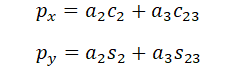
By adding d₁ to the Y coordinate, as we mentioned before, we have the final position equations:

Now we can create a new script to compute these equations and display the manipulator's workspace. We'll do that by iterating all the possible joint angles and calculating the corresponding positions. Since the joints are not free to rotate 360 degrees, we have to incorporate the limitations in our algorithm. For our robot, the joint limits are:
And here's our script:
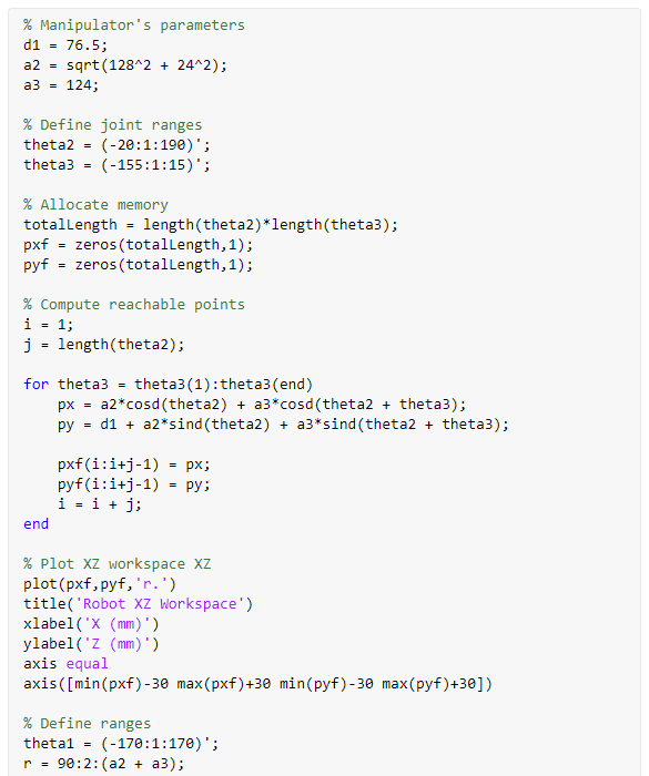

Notice that it's divided into two parts. First, we calculate the workspace for the XZ plane, which depends only on the ranges of θ₂ and θ₃. Then, we compute the YZ workspace, which is a ring and depends on the range of θ₁. Of course, when θ₁ is not zero, the position won't lie in the XZ plane anymore, but in another XYZ plane with the exact same workspace shape.
Here are the results:


It's important to realize that this workspace calculation is not accounting for everything. When we develop the inverse kinematics algorithm, we'll have to add more restraints, for example, for the robot to avoid collision with itself and with the base.
3. Inverse Kinematics
There are two approaches to solving the inverse kinematics of a manipulator: the algebraic one, and the geometric one. The algebraic one involves solving equations systems, whereas the geometric one involves decomposing the spatial geometry of the robot into simpler plane geometry and then solving it using mathematical tools, like trigonometry.
We'll solve our manipulator's kinematics using the geometric approach because it's simpler. To do so, we'll divide the problem into two planes: a side and a top one, and from there we'll write geometric equations that describe its positioning.
The problem that we are trying to solve can be described as: given a desired position (XYZ) and orientation (γ), what joint angles place the wrist (and later the tool) there? Note that γ is the angle of the last link with respect to the base plane.
Let's begin by defining the two planes and the variables:
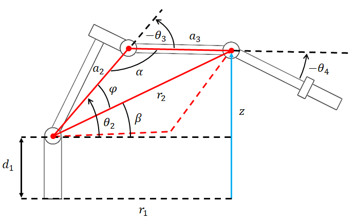
side view

top view
On both views, we have triangles formed by the desired XYZ coordinates, the robot's parameters a₂, and a₃, and the triangles sides r₁ and r₂.
From the top view triangle, we can find the value for the first joint. Notice that we have to use the atan2 function to account for all quadrants:
From that triangle, we can also compute the value for r₁. There, we also have to account for quadrants, because sometimes we'll need r₁ to be negative, so to calculate it we have to use a sine or cosine relationship of the angle we just found instead of the formula of a right triangle based on X and Y:


Moving to the triangle on the side view, we can compute r₂ using the Pythagorean Theorem:

The α angle can be written in terms of θ₃:
Applying the law of cosines to that triangle yields:
Finally, using the cosine identity below, we can write the equation in terms of θ₃:

Here we find our first constraint. Notice that for the triangle to exist, the goal length must be less or equal to the sum of the link lengths, a₂ + a₃. If the goal distance is greater than this, it means that it's out of the manipulator's reach and a solution doesn't exist. Therefore:
This is a condition that we're going to check in our algorithm to determine if a chosen point is reachable. Assuming a solution exists, we have to solve for a value of θ₃ that is between 0 and -180 degrees, because only for these values the triangle exists:
We arrive now in an interesting discussion about manipulators. You can check that for this particular robot, for a desired point, there are two possible solutions. The second one is represented by the dashed line on the side view diagram. We'll call these solutions the "elbow up" and the "elbow down" configurations. In this case, the negative range of θ₃ corresponds to the "elbow up" position. If we'd like to have the other solution, we can find by symmetry that θ₃ would instead have to be positive and lie between 0 and 180 degrees. Here's an example:
elbow up

elbow down
It's also important to realize that as discussed before, we're calculating the inverse kinematics for the robot's wrist. When we go from the wrist frame to the tool frame, which is what really matters, we'll have many possible solutions in each of the two configurations.
To get θ₂, we'll find expressions for the angles β and φ. For β, since we have to account for quadrants, we can write:
To find φ, we apply the law of cosines again to the same triangle:

Here again we have to limit the angle range so that the triangle exists:
We can then compute θ₂ as being:
Where it's +φ for the elbow up and -φ for the elbow down position. On the side plane, the sum of the three joint angles equals the desired orientation γ. With this, we can compute θ₄:
So far we have what we need to compute the inverse kinematics related to the wrist frame. However, in practice, what we want is to compute it for the tool frame related to our application. To achieve this, we have to answer the question: if we want the end-effector at this position and orientation, where does the wrist need to be? By making this transformation, we'll have the desired pose for the wrist that will place the end-effector where we want, and then we can use the equations we derived to calculate it.
Let's see the robot in another pose from which it'll be easy to visualize the desired γ angle:

side view

top view
We'll use the subscript "t" to represent the desired tool or end-effector position. Notice that the γ angle doesn't change, because in our inverse kinematics calculation it was always the angle of the last link (which is the tool link) related to the base frame.
From the side view, in order to obtain the wrist Z coordinate related to the tool position, we have to subtract one side of the triangle from it, thus:
The other side of the triangle, r₃, can be found by:
Moving to the top view, now that we know r₃, we can compute X and Y:

Now we have all the equations to compute the possible joint rates for a desired end-effector position and orientation. Next, we'll implement it on our model and simulate it to check if it's correct.
4. Simulation
We've built a Simulink/Simscape model to simulate our manipulator's inverse kinematics. As input, we have the desired position (X Y Z), orientation (angle), and the elbow configuration (up or down). We also have the gripper opening and closing mechanism as before, but that is not relevant to this problem. We've also added two lamps to show if the desired pose is reachable or violates any joint constraint:
MODEL 1

Here are the rest of the blocks:
Desired Position (desPos)

Goal Representation

Wrist Representation

Simscape Model


And here's the Matlab function that calculates the inverse kinematics using the equations that we derived:


As outputs, we have the joint angles and also a 2-element logical vector indicating if the point is reachable and if the angles are within the available range.
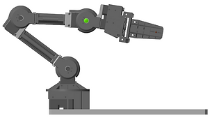
Next, let's run the simulation. An orange ball will represent the desired end-effector position, and a green one will represent the required wrist position in order to achieve that:
We can see that our algorithm works quite well. The end-effector goes to the desired position and orientation. Next, we'll run a simulation with a side view and Y = 0 so that we can better visualize the two elbows' possible positions. In this run, we'll turn off the joint constraints so that we are not limited. Otherwise, it would not be able to reach the same pose in both configurations due to joint limitations.
Near the end of the simulation, we also show how it's possible to reach the same point with many different orientations. For example, below the end-effector is placed in the same position, but with different orientations:


Next, we're going to build a different algorithm. In this one, we'll always try to keep the orientation at 0 degrees. When that's not possible, we're going to iterate until we find the nearest orientation where the pose is achievable. The multibody model remains the same, the only thing that changes is our inverse kinematics algorithm. We've also added a switch to open and close the gripper:
MODEL 2

Here's our new function:


And the simulation:
This model is not so raw as the first one. We have added checks for joint constraints and collision avoidance with the ground and the manipulator itself.
The next and final model that we'll create in this chapter, is the one to pick up and drop off an object. To achieve this we'll also use Stateflow in our model:
MODEL 3

(click to enlarge)
All the functions and the multibody model remain the same. The only addition is the Stateflow chart and the buttons that we'll now use to increase the robot's position in a given direction, instead of directly going to a chosen one as before.
Here's the model for our target:

And the Stateflow:
Main chart

Pick Up chart

Drop Off chart

Where tx, ty, and tz are the target XYZ coordinates.
In this model, the manipulator and the target start at an initial position. We can move the end-effector in space using the buttons and pick up the target whenever we want by clicking the switch. The manipulator will first move to a safe position above the target, stop, and then proceed to pick it up. Once it's picked, we are free to move the robot again, which is now holding the target. We can then use the switch once more to drop off the target in the current XY coordinate. It's possible to do this as many times as we want. Notice that we've also increased the area of the base in order to have more space where to place the target in this model.
Let's see it running:
The model works well. We can move the robot around easily and it picks and drops the target accurately. This model could further be improved in order to add more functionalities, such as giving specific pick up and drop off coordinates and also intermediate ones, so that the robot follows a path between the first and the last point.
4. Conclusion
In this chapter, we calculated the inverse kinematics for our 4-degrees-of-freedom manipulator and implemented it in three different multibody models. We saw that sometimes that are many solutions to reach a specific position, and implemented logic in our algorithm to try to keep a specific orientation, adapt when it's not possible, and also avoid collision with the robot itself. We also saw how to calculate and represent the workspace of a manipulator. In the next chapter, we'll begin to work with velocity. We'll learn how to calculate it for the end-effector, and also do the opposite: compute which joint rates are necessary in order to have a specific one.