ROBOT ARM: PART III
1. Introduction
So far, we have only concerned ourselves with displacement. In this chapter, we'll begin to work with velocities as well. We'll learn how to calculate the linear and angular velocity of the end-effector. This process yields a matrix called the Jacobian, which maps joint velocities to tool velocity, and opens up many possibilities regarding how to control and which tasks a robot can perform. We'll also do the opposite, calculate which joint rates are required in order to have a chosen end-effector velocity. This in the future will allow us to have the robot follow a specific path with a constant linear velocity, resulting in a smooth movement, which is what we want.
2. Velocity propagation
When a robot is moving, each link has a linear and angular velocity at every instant. A manipulator is a chain of connected bodies, where each one of them moves relative to its neighbors. This means that starting from the base, the velocity of each link will be the velocity of the previous link, plus its own velocity. In other words, the velocity of link i + 1 will be the one of link i plus whatever new velocity components were added by joint i + 1.
We are not going to explain here how the velocity equations are derived. For the angular and linear velocity of a link, with respect to its own frame, we have:

where

Notice that the rotation matrices are there to rotate from the current frame i + 1 to the previous frame i, and not the next one, as we have been using them so far. Once we know the linear and angular velocity equation of the last frame, we can write them in terms of the base frame by multiplying them by the rotation matrix that performs this:

We'll write a Matlab script to perform these calculations for us. It calculates the velocity from frame to frame, and then the velocity of the end-effector in terms of the base frame {0}:


Let's take a look at the resultant velocities for each frame:


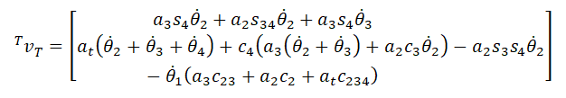
What matters for us, however, are the velocities of the end-effector in terms of the base frame. We can calculate them using the rotation matrix, as mentioned before:
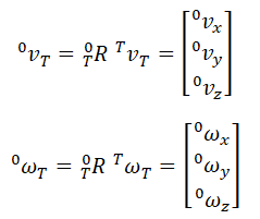
Where each component is:


These equations give us the linear and angular velocities of the end-effector, for known joint rates. Let's implement them in our model to check if they are correct. Here it is:
Main Model

(click to enlarge)
Position Increment

Desired Position Function

Velocities Calculation Function

This function is using the same equations that we just derived in order to calculate the end-effector velocity. Let's run the simulation and see how it goes:
Our calculations and implementation are correct, we can see in the plot that the correct linear velocity increases when we move the end-effector in that particular direction. Let's better see the plot from the simulation in the image below:

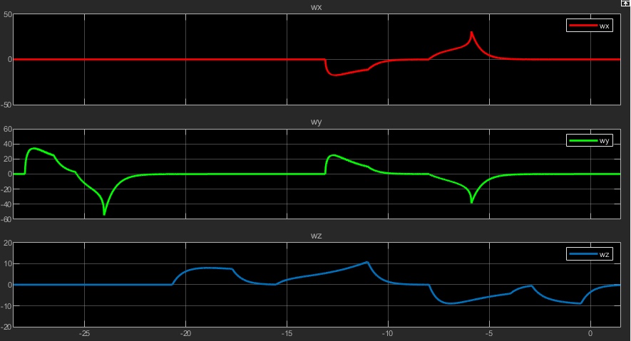
With the current model, we reach a maximum of about 36 mm/s in each direction. We did not simulate enough in order to keep it constant because we didn't want to make a long video, but just show that it works. Now let's run another simulation and look at the angular velocities:
Here the model is also working as expected. At the beginning of the simulation, when we move the end-effector in the -X direction, the angular velocities are 0 because the frame isn't rotating. However, as we approach an area in which the manipulator has to rotate in order for the desired position to be achievable, we notice that the angular velocity in Y, and only in Y, increases, because the frame is rotating around it. Next, when we move it in the +Y direction, we see only the Z angular velocity increasing, which is also what we expect since in that case we are having a translation in XY and a rotation in Z. Finally, as we move it in the -X direction, at first we see a rotation around Z, while in XY we only have a translation, and again when it gets into the zone where it has to rotate in order to achieve the desired position, we see an additional rotation in X and also Y, which is the same thing that happened before, but now we have a rotation in X as well because the tool is not in the
Y = 0 plane anymore. Below you can check the scope:
Next, we'll introduce and talk about the Jacobian matrix.
3. Jacobians
In short, the Jacobian is a matrix that maps velocities in the joint space to those in the cartesian space. The velocity of the end-effector depends not only on the joint rates, but also on the joint angles, as the previous equations clearly show. The Jacobian is a matrix that accounts for those relationships. We define it as:
Where is the vector of joint angles, and is the vector of cartesian velocities. For the general case of a six degrees-of-freedom manipulator, is 6x1, being the 3x1 linear velocity vector and the 3x1 angular velocity vector stacked together. Also for this case, the Jacobian is 6x6, and 6x1. Notice that when we omit the subscript v and w, it means that we're talking about the tool frame:

As you may have already realized, the Jacobian is a way of writing the same velocity equations that we derived before in matrix form. By analyzing the structure of this equation, we see that Jacobians of any dimensions (including non-square) can be defined. The rows in the Jacobian are how many degrees of freedom we are considering, and the columns equal the number of joints that our robot has.
Let's calculate the full Jacobian for our robot. Since we've already calculated the velocities in the previous section, we can just write a continuation of the script to compute the Jacobian from them by transforming from equations form to matrix form:

This yields our Jacobian:

Where:


Now we're going to use it on our model to compute the same velocities as we did before, but with using the Jacobian. The model will be the same, except for the function that computes the velocities, which now will be this one:

Let's run a new simulation and check the results:
It's working as intended, we perform the same movement as before and we can see that the results and like the ones from early. Here are the scopes:

So far we've been able to calculate the end-effector velocity for given joint velocities. But what if we'd like to do the opposite? That's what we're going to see next.
4. Inverse Jacobian
So far we've been able to calculate the end-effector velocity for given joint velocities. But what if we'd like to do the opposite? If our Jacobian is invertible, we can perform this operation and use it to calculate joint rates from desired cartesian velocities:
Since only a square matrix is invertible, we can't use our previous complete Jacobian, which is 6x4. For our application, however, because we keep the tool angle at 0 degrees, we are not trying to control its orientation, but just its position. This means that we can rewrite a square 4x4 Jacobian which will have the XYZ positions that we need and the angular velocity in X, which we do not care about, and invert it. From there we can use the inverse Jacobian or extract the equations for the joint rates and incorporate them into our model.
To compute this, we'll just write another section on the previous script, which calculated the Jacobian:

Since only a square matrix is invertible, we can't use our previous complete Jacobian, which is 6x4. For our application, however, because we keep the tool angle at 0 degrees, we are not trying to control its orientation, but just its position. This means that we can rewrite a square 4x4 Jacobian which will have the XYZ positions that we need and the angular velocity in X, which we do not care about, and invert it. From there we can use the inverse Jacobian or extract the equations for the joint rates and incorporate them into our model.
To calculate this, we'll just write another section on the previous script, which calculated the Jacobian:
And we have our inverse Jacobian:

Where:


In the same way that we transformed equations into the Jacobian, which is the matrix form, we can decompose it from matrix to equations form. That's what we're going to do with the inverse Jacobian. We'll use the joint equations instead of the matrix in our model. The last part of the script does this, and it yields the following results:

Notice that we could just as well use the equation at the beginning of this section to compute the joint rates. Both would give the same result. We just chose to use equations in order for the function to look cleaner. Now let's add it to our model:

(click to enlarge)
Position Representation
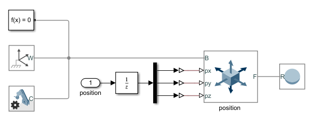
And this is the implemented function:

Now let's run a simulation to see how it performs. A yellow ball will indicate the position of the end-effector:
Our algorithm is working as expected. We are able to move the fingertips in the desired direction with a constant velocity. This is clearly shown when we look at the normal views. This is a very good accomplishment, which will open up many possibilities for.
4. Conclusion
In this chapter, we learned how to calculate the linear and angular velocity of the end-effector. We derived the equations for our manipulator and implemented them in our model. We also did the inverse velocities, that is, calculate the joint rates for given cartesian velocities. We saw how we can compact these equations into a matrix form called Jacobian, and also derived them for our model. In the next chapter, we'll use the inverse kinematics derived until now to implement a path-following algorithm and make the end-effector follow a desired path with a constant velocity.