SELF-BALANCING
MOTORCYCLE: PART I
1. Introduction
In this project, we'll construct and program a motorcycle that balances itself using a reaction wheel:

The basic principle behind this is Newton's third law of motion. Imagine that you're sitting on a rolling chair and there's a desk in front of you. If you push the desk with a certain force, the desk will push you back with a reaction force of the same magnitude and you will slide back. Here the same principle is in place, but instead of linear, we have circular motion. When the motor exerts a torque on the reaction wheel, it will apply an equal torque on the motor in the opposite direction. Since the motor is fixed on the motorcycle's body, the torque will be applied to the whole system, causing it to turn back towards the equilibrium position. Because the wheel applies a "reaction" torque, we call it a reaction wheel or inertia wheel.

motor torque
wheel reaction torque
2. System components
Let's take a look at the system components and then we'll test each of them to make sure that they're working properly before going further into the project.
The wheel is powered by a DC motor fixed on the motorcycle's frame:

We have attached 16 magnets to the wheel using duct tape. The tape is not shown here in the model so that we can see them. We also have a hall effect sensor fixed on the bike's body in a way that when the wheel turns, the magnets pass in front of it. The sensor will generate a pulse each time this occurs, and that will allow us to compute the wheel's velocity.

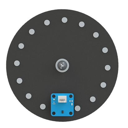
magnet
hall sensor
After successfully building a control system to balance the motorcycle, we'll also be able to drive it back and forth using a geared DC motor:

Motion is transmitted to the rear wheel through a timing belt and pulley:

timing belt
pulley
pulley
This particular motor has a built-in encoder that we will use to calculate the bike's linear velocity.

magnetic encoder
The last feature that we'll implement is to try to steer it. For that, we have a servo motor fixed on the body that will turn the fork left and right up to a maximum angle of ± 35°.


servo motor
We'll use a total of three boards in this project. To handle the system logic, we'll use an Arduino MKR1000 board. This is a Wi-Fi board that will allow us to move the motorcycle wirelessly. To drive the motors we'll be using the MKR Motor Carrier. Finally, to measure the leaning angle and angular velocity we'll use an MKR IMU (inertial measurement unit) which has a 3-axis accelerometer, magnetometer, and gyroscope. As you can notice, all three boards are from the MKR family, which means they have compatible pins and we can just plug one into another. This is a nice thing since it will allow us to use fewer wires and have a compact system.

MKR Motor Carrier
MKR 1000
MKR IMU
In the front, we have an ultrasonic sensor that can be used to detect objects and avoid collisions. We won't be adding this feature to the project right now, but it is a nice option to have in case we want to further develop it, and it also gives a nice motorcycle-looking aspect to the project.

To power the motorcycle we use a 12V battery fixed at the back. Throughout the project we may change its position to align it with the rest of the body. The position below makes the bike more stable but at the same time it gets moved around easily and may change the center of mass of the system, which is not desirable.

battery
3. Testing each mechanism
Next, we'll test each of the components and also the movement of the mechanisms to make sure that they are working as intended.
Let's begin with the IMU. We'll only be outputting the angle and its rate of change (angular speed). The sensor outputs the values in all X, Y, and Z directions. The one that we need is the second one, so we add a selector to choose that index. Also, our convention is that the counterclockwise direction is positive, so we have to add a -1 gain to the velocity output to have it that way. Finally, the status output refers to the IMU's calibration:

To give accurate values, the IMU needs to be calibrated when its first started. The status output refers to the calibration of each sensor (IMU system, accelerometer, magnetometer, and gyroscope). The values range from 0 to 3 and indicate the degree of calibration. For our purpose, we need the accelerometer and the magnetometer to be fully calibrated. It's useful for us, however, to only have one variable (true or false) to indicate if the whole system is calibrated to the degree that we need, so we add a compare to constant block and a sum of products to achieve that:

We wrap this in a subsystem to be used later in the order that's convenient for us (angle, speed, and calibration status):

Now let's test the IMU to see how it works. Notice that the first plot corresponds to the angle, the second to the angular velocity and the third to the calibration status of the sensor (0 = false, 1 = true);
It's working as expected. Let's move on to the next component, the inertia wheel. As we saw earlier, as the wheel turns, the magnets will pass in front of the hall effect sensor, causing it to produce a pulse. When not sensing a magnetic south pole, the sensor outputs 1. When the magnet passes in front of it, it outputs zero. By counting how many pulses we've read in a certain amount of time, we'll be able to calculate the wheel's speed. This is tricky, however, because we need to find the optimal time interval. If the interval between reads is too small, maybe there won't be a pulse, and the calculated speed will be zero, even though the wheel is spinning. If we choose an interval that's too large, we will read a delayed value that will be the average for the whole interval and also won't be able to detect speed changes that may have occurred in between. This will compromise the accuracy of our controller. The choice is based on how often we can read angular displacement (i.e. how many pulses we read for each revolution). In our case, we have 16 magnets, and so we read 16 pulses when the wheel turns one full revolution. It's also important to notice that the greater the interval, the lower the speed step size. For example, with an interval of 100ms we may read the speed in 200rpms increments, whereas with an interval of 50ms for the same setup, we would read it in 400rpms increments. Because our system is discrete and has a fixed time sample of 10ms, the interval will obviously have to be a multiple of that. By trial and error, we select an interval of 80ms between reads. Here's our complete model:

(click to enlarge)
To read the pulses, we need an interrupt pin. This pin will interrupt the execution and outputs its value whenever a falling signal occurs (remember that our sensor outputs 0 when a magnet passes by it). We need it to be an interrupt pin, because otherwise we may miss pulses that happen between reads on our main time sample of 10ms:
pulses

We have a counter that adds 1 every time a pulse occurs.
function()

We pass this to the speed calc block, where by dividing the amount that the wheel has turned by the time interval we compute its speed:
speed calc

So far we have calculated the wheel speed, but we also need to know in which direction it's turning. Part of the logic to doing that is latching, or locking in the first direction it turns when it's first started. From there we can identify direction changes and keep the direction updated. To latch the first direction, we use the logic below. Notice that if we had a board with two hall effect sensors in phase, as is the case with the rear wheel DC motor, we would be able to compute the spinning direction without doing this. In this case, it's not possible because our board only has one sensor.
direction latch

So far we have calculated the wheel speed, but we also need to know in which direction it's turning. Part of the logic to doing that is latching, or locking in the first direction it turns when it's first started. From there we can identify direction changes and keep the direction updated. To latch the first direction, we use this logic:
inertiaWheelVelocity

When the wheel is first started, we know that its direction is the same as the applied motor voltage. From there, we have to identify direction changes. It happens when two conditions are met: first, the desired direction, that is, the current motor voltage value, has to be different from the current direction. This happens when the wheel is decelerating. For example, if the first motor voltage direction was 1, the wheel began spinning in the positive direction. When by any motive we change the voltage to a negative value, the applied torque will change direction, but the wheel will have to decelerate first before beginning to turn in the opposite direction as well. The second condition is that the wheel speed is zero. This means it decelerated and now began turning in the other direction. When both of these conditions are met, we change the speed direction. The third condition in the if statement (desDir ~= 0) is a detail and is only there to prevent the speedDir value from constantly changing when the wheel is stopped. It doesn't affect the logic of the function.
Here we have to go back to the time interval logic used to compute the speed. Because one of the conditions to identify direction changes is that the speed of the wheel is zero, we have to choose an interval that achieves this. If we choose an interval that's too small, this may not happen. That is, we may never read zero speed and therefore this function wouldn't work. Let's see the inertia wheel in action:
We can see that an 80ms interval was a good compromise between accuracy and being able to identify direction changes even when we change the speed from one extreme to the other. Notice also how the motorcycle is pushed to either side when the motor is applying torque in that direction. Here we begin to see the principle by which we'll be able to balance it upward.
Next, let's implement logic to find the linear velocity. Here the logic is straightforward and is the same we've used in other projects. By reading how many encoder pulses there have been between two reads, we can compute the velocity in meters per second:

(click to enlarge)
And here's it in action:
Because our mechanical parts (wheel turning axis and timing belt) don't move very smoothly, we have small variations in our speeds, but that's completely acceptable for our purposes.
The next component that we'll verify is the servo used for steering. We've identified the angle limits as being 35° in each direction, so we want our steering limits to go from -35 to +35°. A servo however operates with values that range from 0° to 180°, so we have to add a bias to the logic to achieve that. Also, we don't want it to instantly turn to the desired angle, as it may cause the motorcycle to lose balance and fall, so we also add a logic to linearly go from the current angle to the desired one. We chose to change the angles in 10° and 15° increments using a rotary switch:

(click to enlarge)
As you will notice, our servo is not very precise and therefore doesn't change position for every 1° increment. It changes more or less at every 10°. That explains the choice for the switch intervals. Also, we're comparing the error to 0.001 instead of zero because for some reason we were not getting absolute values. Let's see it implemented:
Lastly, we want to be able to know the current battery voltage supply. We do not want to run our inertia wheel motor if the read is too low, because then it would not be able to supply torque in the range that our controller was designed and tuned to. Later in the project, we will add logic to not start and turn off the motor if the battery level drops below a certain value. The battery level is originally given as a 32-bit unsigned integer. So we have to add a data change block to convert it to a floating-point number and also divide it by 77 to get the real-world value in volts. In the run below our battery is fully charged and thus providing around 12V:
4. Conclusion
We've tested all the components and created the control logic that we're going to need as we develop the self-balancing motorcycle. We've also seen some limitations of our hardware and how we could overcome them, when possible. In the next part, we'll derive the differential equations of motion of our system, analyze its behavior, and implement a controller to keep the motorcycle upward.