SELF-BALANCING
MOTORCYCLE: PART II
1. Introduction
Now that we know that the components and mechanisms are working as supposed, we can begin to model our system. In this part we'll derive the dynamic equations using two methods: Newton's laws and the Lagrange method, sometimes also called the energy method. We'll verify its behavior and then we'll develop a controller to move the motorcycle around the vertical position.
2. Modeling the system: Newton's Laws
We're going to have to simplify our system before writing the equations of motion. Especially due to the fact that we're going to need to know the moments of inertia of the parts, it would be extremely time-consuming and counterproductive to calculate it for each component. Instead, we'll model the whole motorcycle as being one block with an inertia wheel:

wheel-ground axis

wheel-ground axis
We'll also assume that: the friction between the moving objects is negligible, the wheels' thickness is negligible, and the system can only pivot around the wheel-ground axis. Note that the black and white circles on the image above represent the center of mass of each part. The black dot on the inertia wheel is just a mark to visually know its current angular position.
To begin, let's define the vertical position as the origin (angle = 0°) and the counterclockwise direction as being positive for the rotation of both the whole system and the inertia wheel. Let's also call the wheel-ground axis, the block axis, and the inertia wheel axis A, B, and C, respectively.

A
B
C
The first approach that we are going to use is Newton's second law that says that the sum of all the forces acting on an object is equal to its mass times its acceleration, or in the case of rotating objects, the resulting torque is equal to the moment of inertia times the angular acceleration.
When the motor is turned off and is not applying any torque on the inertia wheel, the forces acting on our system are the weight of the body and of the wheel, which we'll call Fb and Fw. In the same way, we'll call the masses mb and mw:
A
B
C
These forces cause the system to turn around the A-axis, so it's useful for us to work with torques instead of linear forces. To calculate the resulting torques, first we have to decompose the forces, since we want to find the one that is applied perpendicular to the system.
A
B
C
The vertical components that go through the center of mass do not contribute to the resulting torque, so we can discard them for this purpose:
A
B
C
Finally, to find the torques, we multiply the perpendicular components by their respective distance from the pivot axis A. In the diagram below, we replaced the forces with the torques applied to the joint.
A
B
C
Now that we know the forces (ie. torques) acting on our system, we'll proceed to derive the equations of motion using Newton's second law. But before we do, you may have noticed that we didn't include the motor torque on the system yet. That's because since it's a principle of action and reaction, as we've said before, the motor torque will be present in both parts, the body and the inertia wheel, with the same magnitude but different directions, and therefore it's easier to include them later in the free-body diagrams. But if that's the case, couldn't we say that the net torque from the motor would be zero and therefore wouldn't have any effect on the system?
Well, this is a tricky problem to understand and even to explain, because although the two parts are "connected" by the motor shaft, they work as independent bodies. When they are falling, there is no weight force interaction between the body and the wheel on that joint. The only force on that joint is the centripetal one which constricts the movement of the wheel around the A-axis. It's as if the two bodies were free-falling. In fact they are, but with the movement constricted to the axis A. This understanding is crucial because it's from this that we'll write the equations of motion without taking into account these other forces that don't exist. Regarding the motor torque, it doesn't net to zero because the two bodies are not really "connected" or constrained to each other when it comes to their rotations. To make it more intuitive, we can think of the "linear version" of this situation mentioned before, which is when we push a heavy object in front of us while sitting on a rolling chair. In this case, we would go away from the object and therefore would not be able to push it again. But in the "rotational version", the heavy object is always there to be "pushed" again, or in this case, rotated again. As it's obvious, the heavier the object, or in our problem, the greater the moment of inertia, the greater the reaction force.
There are also other particularities regarding this problem that we'll take into account later in the project. For example, we want to make sure that the center of gravity of the system always corresponds to the angle zero, because otherwise the system would be trying to balance around a position where torque due to gravity is present. This means that the motor would need to provide a constant torque to net the sum of torques to zero and balance the motorcycle in place. With a constant torque applied to it, the wheel would accelerate to infinity, which in the real world is obviously impossible because something would break first. In this case, it could be the motors overheating due to the constant electric current, or some other problem related to the friction between the components.
With all this explained, we can proceed to the equations. When we draw free-body diagrams for linear forces, we usually break the dynamics into cartesian coordinates to make it easier. Basically, we sum the forces acting on each body in a particular direction (X, Y, or Z). For circular motion, instead of diving it into directions, the equivalent is to divide the problem into axes of rotation. That means that we'll sum the torques making that object turn around a particular axis. The body only revolves around the ground axis. The wheel, however, turns around both the ground and its own axis, so it'll have two initial equations, making a total of three. We'll then sum two of them to get our two main dynamic equations that are needed to describe the system behavior, since it has two degrees of freedom.
From Newton's second law, we have that the sum of the torques acting on an object rotating around a particular axis is equal to its moment of inertia in that axis times its angular acceleration around that axis:
Let's begin with the free-body diagram of the body rotating around the A-axis. The torque on this axis is the one from gravity that we calculated before. However, now we'll also introduce the motor torque. This reaction torque will be applied in the opposite direction and is the torque that will take the motorcycle back towards the vertical position:
For the wheel, regarding its rotation around the A-axis, we also have the torque due to weight. The wheel revolves around this axis with the same speed as the body:
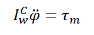
On the axis that passes through its center of mass, the applied torque is the motor torque:
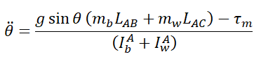
These are our first three equations of motion. Next, we'll sum the first and the second equations, since they both are a function of the angular displacement theta. This gives us the two equations that we need:

Replacing the torque equations from earlier in the first equation finally yields:

Notice that we have three different moments of inertia: the one for the body around A, the one for the wheel around A, and the one for the wheel around C. Let's calculate them.
Starting with the wheel, the moment of inertia of a disk with a radius r rotating around its own axis C is:

From the parallel axis theorem, we can compute its moment of inertia around A:
To find the moment of inertia of the body around A, first we need the one around its own center of mass, the point B. For a rectangular parallelepiped this is:


d
h
Using the parallel axis theorem again, we find its moment of inertia around A:
The equations highlighted in blue are the ones that we are going to use. We won't replace the moments of inertia into the differential equations to get two giant ones. We'll compute them like this using software in order to keep the logic clean and easy to read.
3. Modeling the system: Lagrange's Equations
Now we are going to derive the dynamic equations using the energy method. The result, obviously, is going to have to be the same. In this method, instead of working with forces, we'll calculate the total energy (potential and kinetic) of the system and then use Lagrange's equation to write the equations of motion.
The so-called Lagrangian (L), is the difference between the kinetic (T) and the potential energy (V) of the whole system:
After calculating it, we use it in Lagrange's equation below in order to write the differential equations governing the movement of the system:

Here, q is a generalized chosen coordinate, and Q is a generalized force associated with q. In our case, we'll have two generalized coordinates because our model has two degrees of freedom.
We can expand this equation so that it becomes easier to visualize and apply the derivatives to each term:

For mechanical systems, the second term is always zero since potential energy is not a function of time or velocity. We have as final equation, then:

The kinetic and potential energy of each body, considering the pivot point A as the ground are:
Kinetic


Potential
Which gives a total for the system of:
Kinetic
Potential

As generalized coordinates, we choose the same angles as before. As forces, we have the respective torques:
Plugging the Lagrangian and the generalized forces back into Lagrange's equation yields the following for each of the generalized coordinates:
By rearranging the first one in terms of the angular acceleration, we finally find:

Which are the exact same two differential equations obtained using Newton's laws.
4. Transforming to state-space
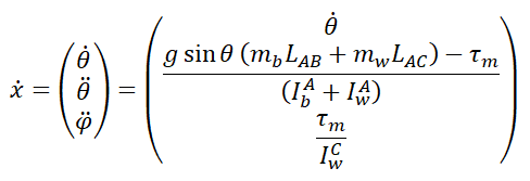
With the equations in hand, we'll proceed to bring it to state-space format. Our chosen states variables will be the motorcycle leaning angle, angular speed, and the inertia wheel speed:

Because of the sinθ in our first equation, it's not linear. We're not going to linearize it before implementing it. Simulink will run it numerically. What we'll do is calculate the derivative of each state using the equations, and then integrate them to find our state variables. By rearranging the dynamic equations we can get :

And the derivative of our state vector becomes:
We'll be using Simulink to run both the simulations and the real hardware. Here's the above model implemented there:

(click to enlarge)
Notice that as we've mentioned before, we calculate the variables using the differential equations and then integrate them to find our state variables. Inside the integrator's blocks, we can set the initial conditions. For this first simulation, we'll set the initial leaning angle to 4, and the body and inertia wheel velocity to 0. Our equations work with radians, so we have to convert that from degrees:

We've also added a simple function to plot and visualize the system's behavior:

To get the system parameters we create a script that load the constants into the workspace:

And in the model we set it to be run after its loaded:

Right now the motor torque is set to zero. Let's see how it behaves when there is no input. Besides the plot function, we're also going to log the state variables in the Data Inspector so that we can check it.
Because we didn't add the physical constraint of the floor to the system, it behaves like an inverted pendulum free to rotate 360º around the wheel-ground axis. Let's analyze the data inspector results:

This is exactly what we were expecting. As there's no energy loss on the system due to friction or other forces, it keeps oscillating. Notice that it reaches maximum speed when it's at 180º, which is the point where it's been accelerated to maximum speed by gravity, and minimum speed at 4º and 356º, which is also what we expected.

max speed

min speed

base angle
There is one thing that we have to change in this model, though. As you can see, the reaction wheel velocity is always zero, which is correct, since we're not considering friction on its rotation axis and the motor is turned off. This, however, is its absolute velocity, relative to the ground. The one that we'll be measuring with our hall effect sensor is its relative velocity with respect to the motorcycle's body, where the sensor is attached. Let's illustrate it below:

initial position

later position
In the initial releasing position of 2º, the inertia wheel is aligned with the body. Later, by the facts mentioned before, it's still in the same absolute position. The magnets attached to the wheel, however, will have passed in front of the hall sensor attached to the body, not because the wheel moved, but because the body did, and we'll read a velocity that won't be zero. This relative velocity is its absolute velocity minus the body velocity, or:
Since this is the velocity that we'll be reading, it makes sense to replace it in our equations. By doing it, the equation for the rotation of the wheel around its own axis becomes:

Our derivatives vector then is:

And here's the updated model:
(click to enlarge)

When we simulate the free-rotating model again, the wheel velocity should have the same magnitude but different direction than the body's. Notice that throughout the rest of the project we'll calculate the wheel speed in RPMs since its more practical, but here just to show this we'll log it in deg/s:

Now we have a model that reads the data like the real-world one that we'll build and we have seen that it's behaving as expected.
5. Controller
The next step is to implement a controller to make it self-balance. In this case, we'll implement a full-state-feedback control based on state error:

Since our reference is zero for all the states (i.e. we want the motorcycle to stay upright at 0º, we want its angular speed to be zero, and we also want the reaction wheel speed to be zero), the values that we read from the sensors are already the state error for each variable, so we don't have to subtract it from the reference value r, which in this case is zero. Therefore, all that we need is to add a gain matrix to our system. Below is the new model. Notice how the state vector is now fed to our controller (or gain matrix):

Here's the updated motorcycle plant:

(click to enlarge)
Now we're joining the states together using a Mux block and outputting it. This is our state vector. We didn't mention this before but notice that while our plant works with radians, the state vector values that will be fed to our controller are in degrees. We do this because the values that we'll read from the IMU will also be in degrees, and it's also more intuitive to work with degrees than with radians. The processing and plotting block contains the plotting function, whose visualization can now be turned on and off using the dashboard switch on the main tab:

We've made a few changes to the original function in order to add this functionality, here's the new one:

Let's begin by adding only a gain to the leaning angle theta and see how it behaves. In the gain matrix, we add another 1e-2 gain so that we can work with integer values rather than with decimals. The first Kp gain will be 1:

Let's see how it goes:
It oscillates between 4º and -4º. When it's at the maximum leaning angle, the applied torque is maximum, since it's proportional to theta, and the system gets momentum. When it gets close to the equilibrium position of 0º, it's moving too fast and so it overshoots and the process keeps repeating itself.

Now let's add a gain to the motorcycle's angular speed. This is a derivative gain since speed is the derivative of displacement. We'll use a value of 0.1:

And here's the result:
The derivative term reduces the actuator's (in this case the torque) command when the motorcycle begins to rotate too fast. With this we got rid of the oscillations and now have a smooth response:

The derivative term reduces the actuator's (in this case the torque) command when the motorcycle begins to rotate too fast. In the opposite direction, we have the torques due to the system's weight. These torques "get to equilibrium" in a way that the leaning angle goes to zero without overshooting. With this, we got rid of the oscillations and now have a smooth response. Just to show the general behavior, a smaller derivative gain, let's say of 0.02, would cause the system to oscillate before reaching the steady-state, as shown below:

So far, we are considering a system that's ideal, meaning that the sensors are perfectly calibrated and a zero leaning angle corresponds to the angle where the weight force passes through the system's center of mass and therefore exerts no torque on the system. Because of this, if we check the reaction wheel speed, we notice that it converges to a finite value when the leaning angle converges to zero, which is acceptable. In the real world, this will never be the case, though. First, because our system is not 100% symmetrical, and second because even if it was, due to the compounding tolerances' errors the center of mass would slightly go to either side. In practice, this would mean that the equilibrium angle for our system would not be at 0º. If that were the case, the system would be trying to balance around a non-zero angle, which means that it would need a motor torque to counteract the weight torque so that the net sum is zero and it stays tilted. This motor torque would keep accelerating the inertia wheel up to a point where something would fail due to overheating, friction, or something else. To sort of simulate this behavior, we can add a bias block to the system to offset the angle. Let's add a 1º offset, which is something we could expect on the real model:

And now let's run the simulation:

Notice how now the inertia wheel speed keeps increasing forever because the steady-state angle isn't zero. This is something that we don't want. To fix this, we'll add a gain to this state as well. Since we're feeding back the velocity in deg/s, which are very high values, the gain will have to be small. In the real model, we'll use RPM instead of deg/s, but since we don't want to go back and change this model now, since it's a simple model only to understand the problem and the system behaviors, we'll keep these units. Let's set a gain of 0.0002:
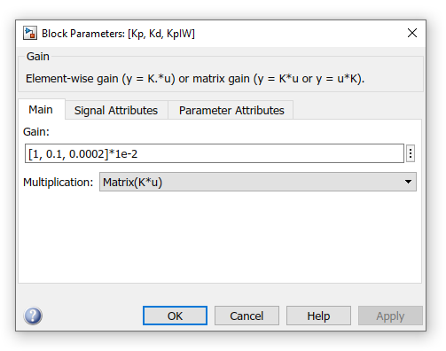
And here's the response:

The reaction wheel speed is now converging to a finite value since our system is balancing around zero like before even though we still have an offset bias. This happens because as the speed increases, so does the motor torque, and it then drives the system to the correct balancing angle. This is the final controller that we'll implement on our real model. Of course we'll better tune the gains in order to achieve an acceptable performance. For example, we probably don't want the reaction wheel converging speed to be very high as it was in this simulation at about 800 RPM, but the general concepts and behaviors will be exactly the same.
6. Conclusion
In this part, we understood the forces acting on our system and derived its equations of motion using two different methods. We made simplifying assumptions and got to a system that is very similar to our real-world motorcycle. This helped us understand its general behavior, and after that, we've developed a controller to balance it. We understood the main points and what possible problems could be on the real model, which is not ideal as this theoric system. There is however another possible approach to modeling this project. Instead of deriving its differential equations, we can use 3D parts and the way they are connected to make a powerful Simulink tool called Simscape do it for us. In this environment, we can simulate its behavior and develop a controller the same way that we did here, with the advantage of not having to derive and work with equations. That's what we'll do in the next chapter.